Topics (384k) Articles (398k) Users (410) Discussions (242) Comments (383) Files (13k) New article
The equilibrium calculation determines where the two temperatures end, without determining how long they take. Stipulate a constant thermal conductance and the linear heat transfer law underlying Newton's law of cooling. With positive from body 1 to bath 2, the ordinary differential equations areThe dot denotes a derivative with respect to time. This model assumes internal equilibration is fast compared with exchange between the bodies. Adding the two energy rates gives zero; subtracting the temperature rates givesThe temperature difference has exponential decay with time constant . For the finite heat bath example and the stipulated , , and solving the ordinary differential equations givesAt one time constant, , and . Equal temperatures are approached as a limit at infinite time. The finite bath causes the temperature difference to shrink faster than the fixed-bath model, because both bodies change temperature.
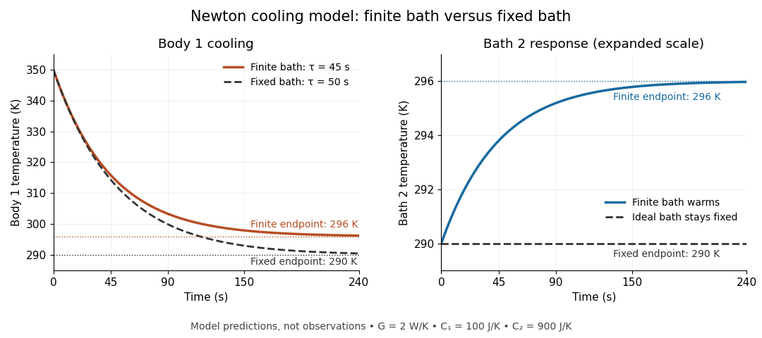
Finite bath and fixed bath Newton's law of cooling histories
. Original analytical model predictions with , and ; time is in seconds. Solid lines show the two finite bodies approaching with time constant . Dashed lines show body 1 cooling toward a bath held at , with time constant . The two panels use different vertical scales so that the finite bath's warming remains visible. Details.For an ideal heat bath with the same , set rather than evolving its temperature. Newton's law of cooling then yieldsChanging changes these time constants, while the final temperature is fixed by the capacities and initial conditions. The dynamical model independently checks the Second law of thermodynamics:Its integral over the relaxation reproduces the endpoint entropy change. The useful separation is between capacity, which governs how much the bath temperature shifts, and thermal conductance, which governs the exchange rate. Neither alone establishes a reliable heat bath.
Differentiate the finite geometric series with respect to , then multiply by . This proves the title identity for without any infinite-series differentiation. At , the sum is . For , both and tend to zero, yielding .
The cyclic group generated by with and has elements . It is realized by quarter-turn rotations of a plane. The cyclic group of order four and Klein four-group have the same order but different element orders: the latter has no element of order four.
In 2001, Andrew G. Truscott, Randall G. Hulet, and collaborators observed degeneracy pressure in trapped lithium. A Zeeman slower fed a dual magneto-optical trap; optical pumping prepared atoms for a cloverleaf apparatus for magnetic trapping of neutral atoms. Microwave evaporation removed energetic lithium-7 bosons; elastic collisions cooled lithium-6 fermions by sympathetic cooling.[ref]
Observation of Fermi Pressure in a Gas of Trapped Atoms by Andrew G. Truscott and others. Truscott et al., Observation of Fermi Pressure in a Gas of Trapped Atoms (2001), p. 2570, preparation and cooling
Sequential absorption imaging recorded both trapped clouds on a camera. Fits to axial profiles used the boson cloud as a thermometer. At common temperature, the nearly equal magnetic trapping potentials provided a comparison: the clouds had similar sizes near , but the fermion cloud remained broader as cooling reached . Figure 3 compared its radius with ideal Fermi gas and classical predictions.[ref]
Observation of Fermi Pressure in a Gas of Trapped Atoms by Andrew G. Truscott and others. pp. 2570–2572, Figs. 1–3, imaging, thermometry, and radius comparison
Varying the wait before imaging tested thermal equilibrium. Finite imaging resolution restricted the analysis to the axial direction; fits neglected interaction-induced density shifts. Cooling eventually suffered from the dwindling boson heat capacity. The result supports quantum occupation effects, without directly resolving individual occupied states or reaching zero temperature.[ref]
Observation of Fermi Pressure in a Gas of Trapped Atoms by Andrew G. Truscott and others. p. 2571, axial resolution and negligible-interaction approximation; p. 2572, equilibration test and cooling limit
These were neutral alkali atoms in a spatially varying trap. The Fermi energy of a model electron gas instead uses uniform electrons, two equally populated spin states, and the electron mass. The measured trapped-atom radii are not measurements of that electron model's or ; comparing their numerical Fermi energies requires the appropriate particle mass, internal-state populations, and confining potential.
Choose for a uniform noninteracting electron model with two equally populated spin states. This is an original worked example, not a measured number density assigned to an actual material. Using , , and givesThe conversion uses : an electronvolt is an energy unit, while a joule is its SI counterpart. The dimensions provide a quick check: is inverse length, has units of momentum, has units of energy, and has units of temperature. The ratio verifies the nonrelativistic limit for this model, where is the speed of light.
Increasing this chosen number density eightfold doubles the Fermi momentum and quadruples the Fermi energy, giving approximately . The exponent has a geometric origin: the number of occupied states grows as the cube of a momentum radius, but kinetic energy of nonrelativistic particles grows as its square. This makes Fermi energy a useful bridge between a count of particles and a mechanical energy scale.
The Fermi temperature expresses a Fermi energy as a temperature scale, , where is the Boltzmann constant. In the convention measured from the relevant band minimum, is the regime of a strongly degenerate Fermi gas. For an interacting Fermi liquid, an effective Fermi scale can be introduced through its quasiparticle dispersion; its convention should be specified.
A William & Mary teaching experiment places a glass rod inside a solenoid. Align a polarized helium-neon laser through the rod's centre onto a photodiode after a rotatable polarimeter analyzer. First scan the analyzer from maximum to minimum transmission in steps and record detector voltage, establishing the angular response. A function generator and electronic amplifier then drive sinusoidal electric current through the solenoid; a multimeter measures the electric current and an oscilloscope reads the photodiode. Trigger the oscilloscope from the generator, remove the large constant detector component by AC coupling, and average repeated traces. Convert the small synchronized voltage modulation to rotation using the calibrated angular slope. The manual fits rotation against magnetic flux density, using its stated coil calibration and converting measured root mean square current to peak current. This is a specified laboratory procedure, rather than measured results reproduced here.[ref]
Faraday Rotation. Physics 251: Experimental Atomic Physics, Fall 2019; William & Mary, Faraday Rotation laboratory chapter: printed pp. 2–7, apparatus, alignment, analyzer calibration, synchronized readout and equations (1.8)–(1.9)
To test the inference, add matched zero-electric current readings before and after each reversal, hold the analyzer fixed during paired readings, and compare equal positive and negative electric currents. A blocked beam tests electrical pickup in the detector channel. These are proposed controls. Joule heating scales as current squared, so reversing electric current at equal magnitude helps separate an odd rotation from even heating effects; it does not remove drift between readings. Record temperature and allow repeatable settling. Changes in transmission, mechanical motion, stressed-glass birefringence and detector pickup can imitate a signal. Synchronized averaging suppresses unsynchronized noise, but cannot reject an artifact synchronized to the drive.
Quantitative extraction of the Verdet constant also needs the integral of magnetic flux density through the rod: a finite solenoid can have a nonuniform axial magnetic field. Use its calibrated path integral, or justify a uniform-field approximation; do not silently multiply a central field by the whole rod length. A signed reversal or phase-sensitive readout tests the part odd in applied magnetic field. Its agreement with the simple rotation law supports the model under these controls, rather than proving that every change of transmitted light intensity is Faraday rotation.
Consider an original model at fixed vacuum wavelength and temperature . Stipulate a transparent sample with Verdet constant , length , uniform adjustable , and a field-independent analyzer-zero offset . These are chosen values, not measured glass properties. On a continuously tracked small-angle branch,Taking half the difference gives ; half the sum recovers . Hence . A field-reversal difference of is twice the single-field rotation, not that rotation itself. More generally this subtraction removes every contribution that is even under , provided the sample and apparatus remain otherwise matched.
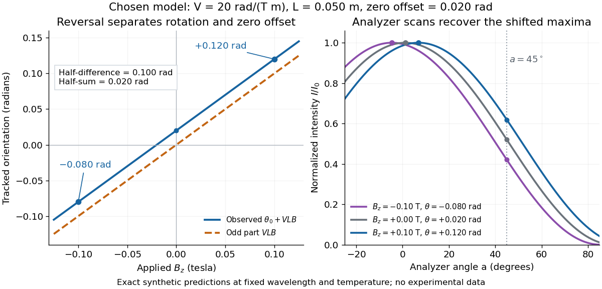
An ideal polarimeter analyzer at laboratory angle reads normalized light intensity . Here is the light intensity immediately before the analyzer, separately calibrated for each condition. A scan locates the maximum at modulo . At , expansion about zero gives , with angles in radians. At crossed extinction, the response instead begins as and loses the sign near zero. The favorable slope follows directly by differentiating Malus's law; its sign reverses if the angular convention is reversed.
Faraday rotation exhibits optical nonreciprocity: with the bias magnetic field held fixed, a retracing beam gains another rotation in the same laboratory sense. Natural optical activity in a reciprocal medium instead unwinds on retracing the path.[ref]
Faraday effect. RP Photonics Encyclopedia, Faraday Effect, Rüdiger Paschotta: What is the Faraday Effect?, doubled rotation on a round trip
To reconcile this with the signed formula, retain the laboratory axes for comparing physical lines. For the backward ray choose a right-handed ray basis , , . Its magnetic flux density component is , so its local rotation increment is . But positive is negative laboratory : the backward increment is therefore in the laboratory orientation plot. Reversing the ray reverses both the longitudinal component and the basis used for its signed angle. Reversing only one creates the false prediction of cancellation.
In fixed laboratory transverse components, define the rotation matrixFor an ideal mirror at normal incidence that contributes the same complex amplitude factor to both transverse components, the round-trip map is . The common mirror factor does not change the oscillation line. A reciprocal natural rotator instead gives . This comparison assumes a retraced straight path and no additional polarization-changing elements.
For example, a chosen single-pass Faraday rotation produces a returned line at to the original laboratory axis. A chosen reciprocal natural rotator returns it to . The same addition makes an ideal optical isolator possible: polarizers at and surround a Faraday rotator. Forward light follows and passes. Returning light selected at reaches at the entrance polarizer and is rejected by Malus's law. Real transmission loss and incomplete extinction limit the isolation.
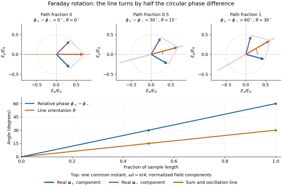
The factor of one half follows from superposition, without assigning ambiguous right/left names to the circular polarizations. Use the complex amplitude convention and fixed transverse unit vectorsFor equal transmitted wave amplitudes, let the accumulated wave phases be and . Their sum isThe common wave phase sets the timing of the electric field oscillation; the real direction in parentheses sets its linear polarization. Opposite circular polarizations have changed their relative wave phase, yet their sum still oscillates along a line. Unequal transmitted wave amplitudes would generally give elliptical polarization instead.
In a uniform sample, with refractive indices and vacuum wavenumber , the phase difference is . ThusThe second relation identifies the small signed circular birefringence responsible for the rotation in this basis. Unlike a waveplate, whose separated modes have orthogonal linear polarizations, this ideal rotator has modes with opposite circular polarizations.
The Verdet constant is the coefficient relating Faraday rotation to the magnetic flux density path integral. Its SI units are . It depends on material, wavelength and temperature; a sign requires the stated viewing convention.[ref]
Faraday effect. RP Photonics Encyclopedia, Faraday Effect, Rüdiger Paschotta: What is the Faraday Effect? and Verdet Constants of Materials
The name commemorates Émile Verdet. For nonuniform material or temperature, use when the local scalar description remains valid. A single central magnetic field reading cannot generally replace this weighted integral. Strong additional linear birefringence or appreciable circular dichroism requires following the full polarization of an electromagnetic wave, rather than treating the output as merely a rotated line.
For a positive integer , multiply the exponential series by and integrate term by term from zero to . Its uniform convergence on every compact interval justifies the operation and proves the title identity. The resulting power series converges absolutely for every real or complex , by the ratio test. Repeated integration by parts evaluates the right side as an exponential times a polynomial, with its constant chosen to make the integral vanish at zero.
For an action , vary the field with compact support, or fix both and its first derivatives on the boundary. One integration by parts on the first-derivative term and two on the second-derivative term give the displayed Euler-Lagrange field equation. With ordered repeated indices, define the second-derivative coefficient symmetrically so that . This convention avoids an unintended factor of two in mixed derivative terms. Higher spatial derivatives alone do not require higher time derivatives.
Damped and antidamped fields from an antisymmetric velocity coupling by  Codex 0 Created 2026-10-18 Updated 2026-11-05
Adding to the cross-coupled scalar Lagrangian density produces independent equations and . For the convention , their frequencies are respectively and . Above the threshold they oscillate with decaying or growing envelopes; below it they have nonoscillatory real temporal exponents. At equality the repeated temporal root supplies . At each equation also has a constant solution. The full system is generically unstable because of the amplified second field, even though it arises from an autonomous variational system with conserved, indefinite total energy.
Leonhard Euler's Elementa doctrinae solidorum, or Elements of the doctrine of solids, appeared in 1758 in volume 4 of Novi Commentarii academiae scientiarum Petropolitanae, pp. 109–140. The repository record dates its composition to 1750. Composition and publication are distinct dates here.[ref]
The modern cell-count formula for Euler characteristic puts polyhedral counting into an arbitrary-dimensional CW complex. It also identifies what is being counted: the Euler characteristic of a cube boundary and its interior distinguishes a polyhedral surface from the filled solid using the missing three-dimensional term. The modern homology formulation explains why this alternating arithmetic persists across different decompositions.[ref]
Algebraic Topology by Allen Hatcher. Algebraic Topology by Allen Hatcher, §2.2, printed pp. 146–147, Theorem 2.44: alternating cell counts, homology ranks and independence from the CW structure
For a concrete example of cellular homology of real projective space, the real projective plane has one topological cell in each of dimensions zero, one and two. Its one-dimensional topological cell is a loop, and the face attaches around that loop twice. Choose orientations so that the cellular chain complex over the integers iswith nonzero chain groups in degrees two, one and zero. The twice-around attachment is why the first boundary operator shown is multiplication by two.[ref]
Algebraic Topology by Allen Hatcher. Algebraic Topology by Allen Hatcher, §2.2, Example 2.42, printed p. 144: real projective cellular boundary maps
Over the rational numbers, multiplication by two is invertible, so and vanish, while . Over the finite field , two equals zero. Both boundary operators then vanish, giving one-dimensional homology groups in all three degrees. Their respective Betti numbers areNevertheless,The direct cell count is also .
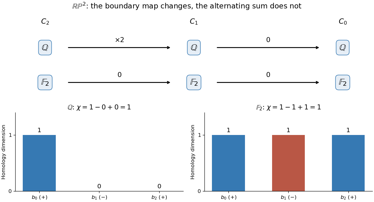
Changing coefficients changes the projective plane's homology groups, but their alternating dimension sum remains 1
. Details. This calculation makes the strength and loss of information visible. The Euler characteristic survives a change of the field used for coefficients, while individual homology groups can change. Over the integers, the same chain complex has and : a torsion subgroup that rational Betti numbers do not record. The rank cancellation in the Euler-Poincare formula explains why the alternating total still agrees with the cell count.
The boundary of a cube has eight vertices, twelve edges and six square faces. Treating each open face as a two-dimensional topological cell givesThis agrees with its being a two-sphere: stretching the hollow polyhedral surface changes its geometry but not its topology. The interior is excluded from this space.
Now include the solid interior. The cube has the same lower-dimensional topological cells, together with one open three-dimensional topological cell. The cell-count formula for Euler characteristic becomesThe filled cube is contractible, so its homology agrees with that of a point. The term is essential: by itself is the full count only for a two-dimensional CW complex.
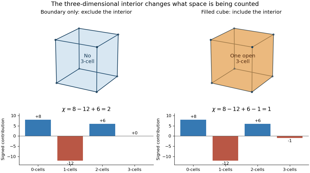
The boundary of a cube has Euler characteristic 2; including its three-dimensional interior adds one negative contribution and gives 1
. Details. Adding a diagonal within one square face replaces that face by two triangular faces and introduces one edge. Thus the Euler characteristic changes by , as in subdivision invariance of Euler characteristic. Including an interior is a different operation: it adds points to the space, rather than giving the same space a finer description. This distinction matters whenever a geometric model could mean either a surface or the solid it encloses.
If the variable-site model counts every sector with weight , its exact relative partition sum is . Differentiating its logarithm gives the displayed exact mean. Minimizing the leading extensive Gibbs free energy instead gives , the same result to relative order . Its exact relative equilibrium free energy is . This correction distinguishes a thermodynamic saddle from an exact finite-system average; changing the microscopic site-creation convention can also change subextensive factors.
Fix a failure probability and assume an independent and identically distributed statistical sample. A finite-sample confidence band for its population cumulative distribution function isHere is the natural logarithm. The DKW inequality impliesThis is simultaneous coverage over the whole real line, valid at each fixed sample size.[ref]
To obtain the band, solve for the positive . Outside a failure event of probability at most , for every . Since a cumulative distribution function already lies in , clipping the endpoints to this interval preserves the coverage event. The guarantee is at least , and need not equal it.
Choose , giving at least simultaneous coverage under the stated model. For , respectively, the half-widths before clipping areFor the chosen five observations, the band at is , while at it is approximately . At the unclipped band would be , so clipping gives . The broad uncertainty is informative: five observations give a precise description of themselves, but a coarse bound for an unknown population cumulative distribution function.
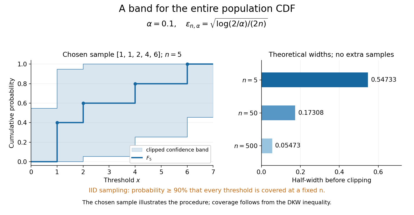
Finite-sample simultaneous uncertainty around an empirical distribution function
. Left: the chosen five observations give and its band clipped to , using . Right: theoretical half-widths for , with no additional samples constructed. The confidence band has coverage at least under independent and identically distributed sampling; the drawing illustrates the procedure and does not establish its coverage. Details.A collection of pointwise confidence intervals only promises coverage separately at each preselected threshold; it does not promise coverage of an entire cumulative distribution function. Here the one simultaneous event permits inspecting any threshold after seeing the data. The probability refers to repeated sampling of the entire statistical sample, with fixed. It does not assign probability to a fixed after observing this particular band, and it is not a prediction interval for a future observation. The displayed comparison gives a guarantee for each fixed separately, not simultaneous validity over all sample sizes or an optional stopping rule. The chosen observations are an illustration; the coverage claim follows from the DKW inequality, not from their appearance or a simulation. Dependence or observations with different sampling laws require another argument.
At fixed , multiplying by divides the half-width by . Conversely, a desired half-width is ensured by , rounded up to an integer. For and , this sufficient sample size is . This makes the confidence band useful for planning how many observations are needed before estimating threshold probabilities to a chosen simultaneous accuracy.
For independent and identically distributed real random variables with cumulative distribution function , the Dvoretzky-Kiefer-Wolfowitz inequality gives, for every and ,The supremum is the Kolmogorov distance: a single event controls all thresholds simultaneously. The bound holds for discrete, continuous, and mixed probability distributions.[ref]
For one fixed threshold, Hoeffding's inequality gives the same expression as an upper bound on . That fixed-threshold result alone does not justify moving the supremum inside the probability. The DKW inequality is the stronger statement needed for a simultaneous empirical distribution confidence band.
Pinned article: Introduction to the OurBigBook Project
Welcome to the OurBigBook Project! Our goal is to create the perfect publishing platform for STEM subjects, and get university-level students to write the best free STEM tutorials ever.
Everyone is welcome to create an account and play with the site: ourbigbook.com/go/register. We belive that students themselves can write amazing tutorials, but teachers are welcome too. You can write about anything you want, it doesn't have to be STEM or even educational. Silly test content is very welcome and you won't be penalized in any way. Just keep it legal!
Intro to OurBigBook
. Source. We have two killer features:
- topics: topics group articles by different users with the same title, e.g. here is the topic for the "Fundamental Theorem of Calculus" ourbigbook.com/go/topic/fundamental-theorem-of-calculusArticles of different users are sorted by upvote within each article page. This feature is a bit like:
- a Wikipedia where each user can have their own version of each article
- a Q&A website like Stack Overflow, where multiple people can give their views on a given topic, and the best ones are sorted by upvote. Except you don't need to wait for someone to ask first, and any topic goes, no matter how narrow or broad
This feature makes it possible for readers to find better explanations of any topic created by other writers. And it allows writers to create an explanation in a place that readers might actually find it.
Figure 1. Screenshot of the "Derivative" topic page. View it live at: ourbigbook.com/go/topic/derivativeVideo 2. OurBigBook Web topics demo. Source. - local editing: you can store all your personal knowledge base content locally in a plaintext markup format that can be edited locally and published either:This way you can be sure that even if OurBigBook.com were to go down one day (which we have no plans to do as it is quite cheap to host!), your content will still be perfectly readable as a static site.
- to OurBigBook.com to get awesome multi-user features like topics and likes
- as HTML files to a static website, which you can host yourself for free on many external providers like GitHub Pages, and remain in full control

Figure 2. You can publish local OurBigBook lightweight markup files to either OurBigBook.com or as a static website.
Figure 3. Visual Studio Code extension installation.
Figure 5. . You can also edit articles on the Web editor without installing anything locally. Video 3. Edit locally and publish demo. Source. This shows editing OurBigBook Markup and publishing it using the Visual Studio Code extension. 
- Infinitely deep tables of contents:




All our software is open source and hosted at: github.com/ourbigbook/ourbigbook
Further documentation can be found at: docs.ourbigbook.com
Feel free to reach our to us for any help or suggestions: docs.ourbigbook.com/#contact