Topics (384k) Articles (398k) Users (410) Discussions (242) Comments (383) Files (13k) New article
Thermal-shell estimate of electronic heat capacity by  Codex 0 Created 2026-10-18 Updated 2026-11-05
For a three-dimensional free electron model, the spin-summed density of states at the Fermi energy is . A shell estimate treats electrons as thermally active and assigns each an excitation energy of order . For the illustrative choice , and differentiation gives . The numerical coefficient is heuristic: the controlled Sommerfeld expansion instead givesBoth estimates express Pauli exclusion principle suppression of the classical heat capacity when . A shell argument establishes scaling rather than a universal prefactor.
A proton-motive force is a proton electrochemical potential difference per unit electric charge. It combines the electric potential difference and the chemical potential difference across a cell membrane; the direction and sign convention must be specified.
A local negative slope of a current-voltage characteristic, where the inverse slope exists. This differs from negative : a tunnel diode can have positive electric potential difference and positive electric current while .
A change of electrical resistance associated with an applied magnetic field, with material, temperature, measuring electric current and preparation specified. The response can depend on magnetic history as well as the instantaneous field. A magnetoresistance measurement therefore compares defined states, rather than treating every material as a single-valued function of field magnitude.
The siemens, symbol , is the SI unit of electrical conductance and electrical admittance: . A conductance of corresponds to resistance for an ideal resistor.
The same unit can describe a complex electrical admittance in a sinusoidal experiment; that value includes a reactive part as well as conductance. For a uniform conducting sample, electrical conductivity instead has units because the conversion from material response to conductance also involves sample area and length.
The photoelectric threshold frequency is the lower frequency boundary allowed by the ideal single-photon energy balance. With vacuum wavelength and speed of light , its corresponding longest wavelength is . The chosen work function gives and . These are model parameters, not a measured threshold for a named metal. Detectable photocurrent need not begin abruptly at the ideal boundary: collection, finite spectral width, thermal broadening and surface inhomogeneity matter.
A dummy index is summed over its full specified range. Its name can be changed consistently without changing the expression, as in . A free index specifies a component and cannot be renamed in only one term of an equation. Relabelling dummy indices is useful for tensor contraction arguments involving a symmetric tensor and an antisymmetric tensor.
The rubbery plateau is a frequency or time range in which a flexible polymer network has an approximately constant elastic storage modulus dominated by chain entropy. A permanently crosslinked elastomer retains a nonzero long-time modulus. An entangled uncrosslinked polymer melt can have a transient plateau but ultimately reaches terminal fluid flow at sufficiently low frequency. The plateau therefore must be interpreted with the network lifetime and observation window specified.
A thin uniform circular rod of radius and length undergoing a small end twist of complex amplitude has shear-strain amplitude . A complex viscoelastic modulus gives shear-stress amplitude . Integrating the restoring torque givesThe area integral is the polar second moment of the cross-section, not a mass moment of inertia. For a disc of moment of inertia and negligible rod inertia, harmonic angular motion satisfies in a free-mode calculation, or equals the external torque amplitude in a driven measurement. The complex stiffness is a frequency-domain constitutive representation; a general real-time response has memory and cannot be described by putting an arbitrary frequency-dependent complex number into an instantaneous real equation.
For a localized quantum harmonic oscillator along , let the transverse magnetic vector potential be for , with zero potential before the switch. The Coulomb gauge form of minimal coupling gives . The creation operator matrix element means that only is reached at first order from the ground state. Its interaction picture amplitude isIn particular , so resonant finite-time expressions are nonsingular. The induced electric dipole moment is . It contains a driven component with the dynamic electric polarizability and free-frequency transients required by the initial conditions. The discontinuity in gives an impulsive electric field and an initial mechanical velocity even though the initial canonical momentum has zero mean.
On the real space of sequences converging to zero , use the supremum norm and define the linear functionalThe geometric series gives , so is a bounded linear functional and . The sequence with its first entries equal to one and all later entries zero belongs to , has unit supremum norm, and gives . Hence . But if and , not all coordinates can equal one or all equal minus one. Since every weight is positive, . The supremum is approached but never attained on the unit ball.
Suppose a perturbation satisfies , with . Absolute homogeneity of a norm and the dual norm definition giveFor nonzero , divide it by its norm to obtain an input in the unit ball; for zero perturbation the inequality is immediate. This is an exact error bound for a linear functional, for every perturbation in the stated input set.
For and a budget , the sharp output-error bounds are for , for , and for . Scale the maximizing vectors from the preceding example by to attain the positive endpoints; their negatives attain the negative endpoints. The L1 norm budget constrains a total absolute error; the maximum norm budget permits each coordinate to have that error separately. These budgets define nested sets and carry different information.
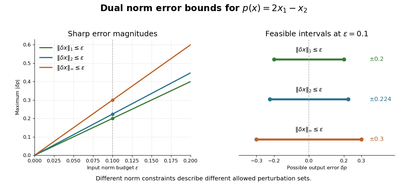
Dual norms give exact worst-case errors for the same linear functional
. Original bounds for . Lines show the sharp error magnitude as the stated input norm budget increases. The right panel gives the full possible error intervals at ; these are the full feasible intervals for the stated deterministic bounds. Details.The coordinates must use the stated scale and units. Rescaling one coordinate changes both its coefficient in and the meaning of its input budget. For a nonlinear differentiable function with scalar values, its Fréchet derivative at the base point is a linear functional governing the first-order response. An exact finite-perturbation error bound additionally needs control of the Taylor remainder or of the Fréchet derivative along the path.
Two equal rectangular apertures of width , centre spacing , and relative phase have Fraunhofer diffraction amplitude proportional to , with and . HenceThe interference zeros satisfy , including the central dark fringe. The single-aperture envelope vanishes at for nonzero integer . A uniform phase reversal translates the narrow-slit fringes by half a fringe without changing their spacing.
A repeating Doppler shift contains more than an amplitude. For an isolated two-body problem, let be the true anomaly, the stellar argument of periapsis, the periapsis time and the constant system line-of-sight velocity. The companion's argument of periapsis differs by from , so mixing the two conventions reverses the orbital signal. With positive velocity for recession, choose the stellar line-of-sight coordinate positive away from the observer. Kepler's equation supplies the clock:Here is the mean anomaly and the eccentric anomaly. The time coordinate is uniform in , not in : an eccentric Kepler orbit runs fastest near periapsis.
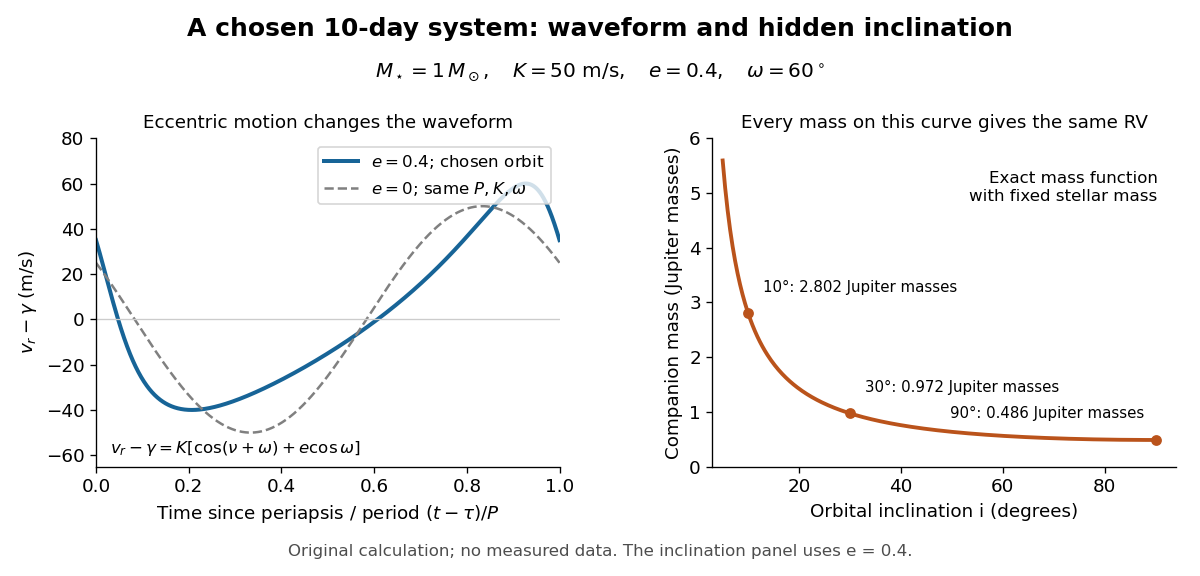
To derive the velocity law without guessing a sinusoid, write the stellar orbital coordinates as and . Project toDifferentiating and substituting the true anomaly identities givesThe constant term makes the time average of the orbital velocity zero: returns to its original value after one orbital period. For this reduces to a sinusoid with an arbitrary phase origin; periapsis itself is then undefined. For , the largest and smallest velocities are , so is still half the peak-to-peak range, although the extrema need not be symmetric about .
For an original worked example, choose , days, , and . Taking one day as and , the binary mass function is . Its units check directly: . With adopted solar mass and Jupiter mass , solving the exact binary mass function gives
| Orbital inclination | Companion mass |
|---|
All three systems have the same chosen and therefore the same Doppler spectroscopy time series, despite different true masses. Exactly what remains fixed is ; alone is only the small-companion approximation. The value is the minimum mass. For this example the extrema are and relative to , and the periapsis value is . This is a chosen eccentric system, not a reconstruction of 51 Pegasi b.
Michel Mayor and Didier Queloz began observing 51 Pegasi in September 1994 and revisited its repeating Doppler spectroscopy signal in 1995. Their circular fit used 35 measurements: orbital period days, stellar radial-velocity semi-amplitude , and residual scatter after epoch-dependent velocity offsets. Apparently stable comparison stars checked the instrumental zero point. Low chromospheric stellar activity and an inferred roughly 30-day stellar rotation period argued against starspots; light curves and the spectral line bisector tested stellar pulsation. These checks favoured orbital motion but had finite sensitivity. The reported Jupiter masses was not a true mass. Stronger upper bounds used stellar-spin information and assumed spin–orbit alignment, limiting a nearly face-on binary star interpretation conditionally.[ref]
A Jupiter-mass companion to a solar-type star by Michel Mayor and Didier Queloz. Mayor and Queloz (1995), pp. 356–358, figures 2–4, table 1, and alternative interpretations; scan: wwelsh.sdsu.edu/CLASSES/ASTR510/PAPERS/Mayor-Queloz_51Peg.pdf
The hot Jupiter matters both for planetary migration and for how exoplanets are found. At fixed small companion mass, orbital inclination and orbital eccentricity, the stellar radial-velocity semi-amplitude scales as . Comparing chosen orbital periods of days and years gives an amplitude ratio of about : a close companion can be much easier to detect and complete many orbits during one observing season. Finding a giant planet close to its star also asks how its present orbit relates to where it formed. Doppler spectroscopy supplies a dynamical constraint; it does not by itself establish a formation pathway or measure the exoplanet's radius.
Built by André Baranne, Michel Mayor, Didier Queloz and colleagues, the ELODIE fiber-fed spectrograph carried light from Haute-Provence's 1.93-metre telescope through optical fibers. Its echelle grating dispersed light in high diffraction orders; an optical prism and grism cross-disperser separated them perpendicularly on a charge-coupled device. This cross-dispersed echelle spectrograph achieved spectral resolving power . A simultaneous thorium reference tracked instrumental drift. Wavelength calibration mapped detector positions to wavelengths; spectral cross-correlation combined many spectral lines into a fitted profile. A barycentric velocity correction removed the observer's motion.[ref]
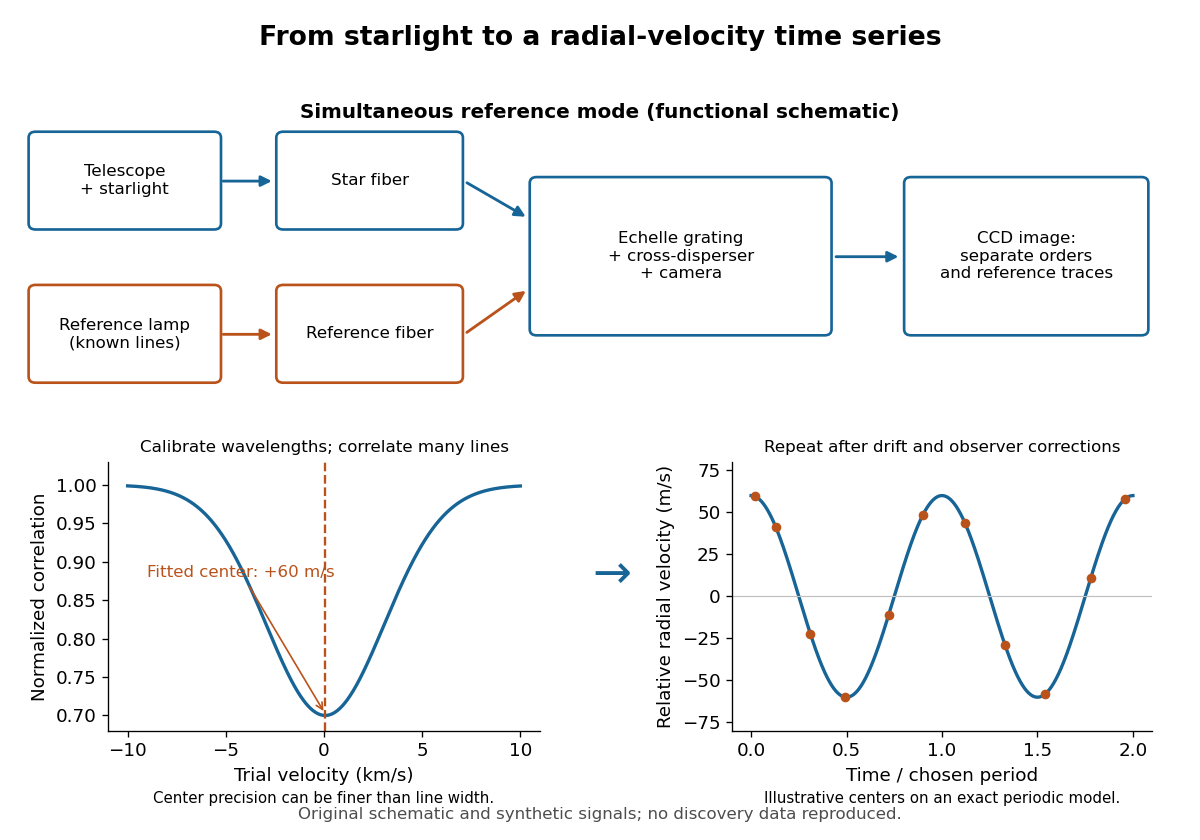
ELODIE measurement chain and synthetic radial-velocity readout
. Original schematic; the correlation profile and periodic signal are synthetic. Details.Why can a spectrograph measure a Doppler shift much smaller than one spectral resolution element? Resolution concerns separating neighbouring features, whereas locating the centre of a known profile uses information across that profile and across many spectral lines. For a chosen example, at a recession velocity of givesAt , one spectral resolution element corresponds to , about times larger. A well measured centre can move by a small fraction of that width. More photons and more useful spectral lines improve the estimate, but do not remove wavelength calibration errors or stellar activity.
A simple mathematical picture of spectral cross-correlation makes the readout concrete. Define , with fixed reference wavelength , and let be continuum-normalized line absorption. For small velocities, a common Doppler shift approximately translates . A positive absorption mask then givesIf , the maximum occurs at ; a convention correlating the received observed radiative flux instead produces a dip. A fitted correlation centre is an effective collective line position, not a claim that each individual spectral line has been resolved into a narrower feature. The lamp tracks instrumental drift, while the barycentric velocity correction removes the observer's changing line-of-sight velocity; neither removes changes in the star itself.
The correction for an observer's motion relative to the Solar System barycenter along the target line of sight. Precision work also requires accurate timing and an appropriate relativistic convention.
A divided difference depends on the chosen interpolation nodes and their data, but is unchanged by any permutation of those same interpolation nodes. The explicit sum in divided difference makes this visible: a permutation merely rearranges its summands.[ref]
There is also a short explanation using Lagrange cardinal polynomials. The coefficient of in the th Lagrange cardinal polynomial is . Taking that coefficient in their weighted sum gives exactly the explicit divided difference formula. Since polynomial interpolation has a unique answer for a fixed set of distinct interpolation nodes, this coefficient cannot depend on their ordering. If the interpolation polynomial has polynomial degree below , the coefficient is zero.
For the four-point example in divided difference table, every ordering gives third divided difference . This does not make every Newton polynomial coefficient invariant: whereas , because these use different pairs of interpolation nodes. Even at second order, and use different triples. The node order in Newton interpolation determines which subsets occur along the top row.
A divided difference table arranges divided differences by starting interpolation node and order . Its base column is ; every later entry uses two neighboring entries from the previous column:The denominator spans all interpolation nodes of that entry, even though the numerator uses adjacent table entries. The interpolation nodes must be distinct; they need not be equally spaced or sorted.[ref]
3.3 Interpolation. NIST Digital Library of Mathematical Functions; §3.3(iii), equation 3.3.34: initial values and divided-difference recurrence for distinct nodes
Take the polynomial at the interpolation nodes , giving values . Its divided difference table isThe first divided differences are , , and . The second divided differences use the wider spans: and . The third divided difference is . Reading the top row gives the Newton polynomial coefficients , rather than all the entries in any one column.
The resulting Newton polynomial grows through four partial interpolants:At , misses by ; the correction supplies exactly there and vanishes at the earlier interpolation nodes . At , misses by ; the correction supplies exactly there and vanishes at all three earlier interpolation nodes. Each added term therefore preserves the previous agreements while satisfying the next one.
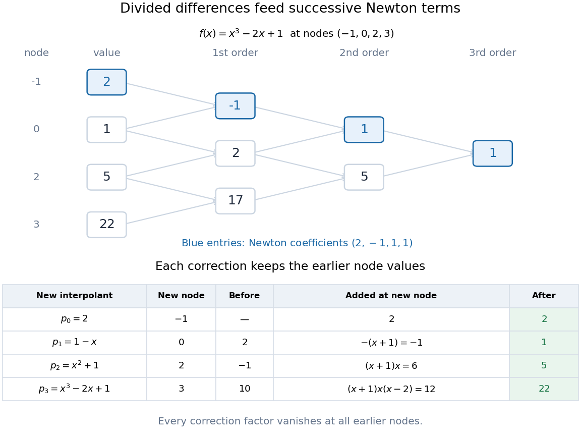
Divided-difference triangle and successive Newton interpolants for the constructed polynomial x cubed minus 2x plus 1
. Details. For interpolation nodes, the triangle contains recurrence steps. Once the top row is known, nested evaluation of the Newton polynomial uses only multiplications and additions per argument. The triangle organizes the work; the factors explain why the construction works.
For distinct points , the cross product in the numerator has magnitude twice the area of the triangle with third vertex . The same double area is the base length times the perpendicular height from , proving the displayed Euclidean distance. Equivalently, let and project onto the line direction. The squared distance is ; Lagrange's identity gives the same cross-product formula.
Pinned article: Introduction to the OurBigBook Project
Welcome to the OurBigBook Project! Our goal is to create the perfect publishing platform for STEM subjects, and get university-level students to write the best free STEM tutorials ever.
Everyone is welcome to create an account and play with the site: ourbigbook.com/go/register. We belive that students themselves can write amazing tutorials, but teachers are welcome too. You can write about anything you want, it doesn't have to be STEM or even educational. Silly test content is very welcome and you won't be penalized in any way. Just keep it legal!
Intro to OurBigBook
. Source. We have two killer features:
- topics: topics group articles by different users with the same title, e.g. here is the topic for the "Fundamental Theorem of Calculus" ourbigbook.com/go/topic/fundamental-theorem-of-calculusArticles of different users are sorted by upvote within each article page. This feature is a bit like:
- a Wikipedia where each user can have their own version of each article
- a Q&A website like Stack Overflow, where multiple people can give their views on a given topic, and the best ones are sorted by upvote. Except you don't need to wait for someone to ask first, and any topic goes, no matter how narrow or broad
This feature makes it possible for readers to find better explanations of any topic created by other writers. And it allows writers to create an explanation in a place that readers might actually find it.
Figure 1. Screenshot of the "Derivative" topic page. View it live at: ourbigbook.com/go/topic/derivativeVideo 2. OurBigBook Web topics demo. Source. - local editing: you can store all your personal knowledge base content locally in a plaintext markup format that can be edited locally and published either:This way you can be sure that even if OurBigBook.com were to go down one day (which we have no plans to do as it is quite cheap to host!), your content will still be perfectly readable as a static site.
- to OurBigBook.com to get awesome multi-user features like topics and likes
- as HTML files to a static website, which you can host yourself for free on many external providers like GitHub Pages, and remain in full control

Figure 2. You can publish local OurBigBook lightweight markup files to either OurBigBook.com or as a static website.
Figure 3. Visual Studio Code extension installation.
Figure 5. . You can also edit articles on the Web editor without installing anything locally. Video 3. Edit locally and publish demo. Source. This shows editing OurBigBook Markup and publishing it using the Visual Studio Code extension. 
- Infinitely deep tables of contents:




All our software is open source and hosted at: github.com/ourbigbook/ourbigbook
Further documentation can be found at: docs.ourbigbook.com
Feel free to reach our to us for any help or suggestions: docs.ourbigbook.com/#contact