Topics (384k) Articles (398k) Users (410) Discussions (242) Comments (383) Files (13k) New article
Define the instantaneous spin magnetization . Global reversal sends to without changing the zero-field energy. Pairing every microstate with its reversed partner proves at every positive temperature, even when almost all probability lies on the two fully aligned patterns. A vanishing mean does not imply weak alignment: the limiting probability distribution is half at and half at .
The Ising ring magnetization fluctuations measure this distinction through variance. In the class, both patterns have . Among the patterns, eight have and four have ; the two patterns also have . ConsequentlyIt equals at , approaches for four independent fair Ising spins at , and approaches as . Unlike the energy variance, the spin magnetization variance remains large in the low-temperature symmetric mixture.
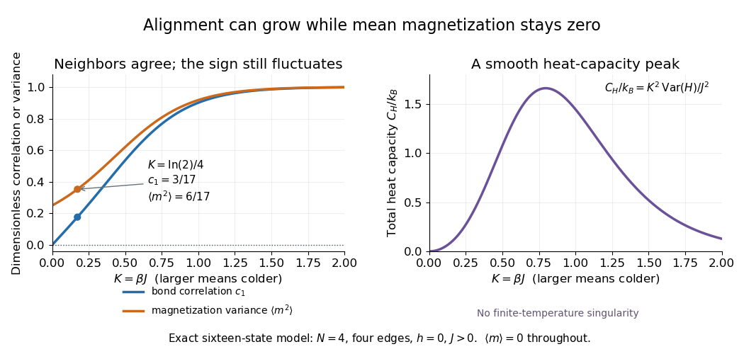
The same thermal fluctuation controls the field response. Allow to vary before setting it to zero; differentiating the Boltzmann distribution inserts , givingThis is a spin-normalized magnetic susceptibility with respect to the energy-valued parameter ; conversion to physical magnetization and magnetic field requires the magnetic moment and sample volume factors.
For finite , is a finite positive sum of exponential functions. Its free energy is a real analytic function for , so the smooth heat capacity peak here is not a critical phase transition. Spontaneous magnetization concerns the order of limits: first a thermodynamic limit, then removal of a symmetry-breaking field. The four-spin Ising ring alone establishes neither that limit nor any two-dimensional Ising model result.[ref]
Statistical Physics by David Tong. §5.2.3, paragraph beginning with the analytic finite partition sum: phase transitions require the thermodynamic limit
The Ising ring bond correlation is the neighboring two-point correlation function in the four-spin Ising ring. All four edges are equivalent. At zero field each mean Ising spin is zero by spin inversion symmetry, so also equals the connected correlation function. Agreement gives bond product and disagreement ; thus .
Differentiating the finite partition function with respect to inserts the sum of four bond products. ThereforeHere is internal energy. At , the class-weight calculation gives and . The agreement probability for a selected bond is , despite the exactly zero mean spin magnetization.
A second derivative gives the energy variance, and hence the heat capacity at fixed and :To see the variance identity directly, a derivative of an expected value under weights inserts , where . The factor follows from . At the same exact example, . The heat capacity vanishes both as and as : at high temperature its dimensionless factor vanishes, while at low temperature excited microstates become exponentially rare.
An th-forbidden beta decay transition with the maximal leading angular-momentum transfer . Only the spin-dependent coupling can attain that transfer at this orbital order. Thus a transition is first-forbidden unique, whereas a same-parity transition is second-forbidden nonunique. Unique refers to the leading weak multipole structure, not a claim that every correction to the decay vanishes.
Immunofluorescence localizes antigens using antibodies and a fluorescence readout. Indirect labeling uses a secondary antibody to detect the bound primary antibody.
A material volume element contains the same fluid particles as it moves and deforms. If its edges transform with the local velocity gradient, its volume changes at a rate equal to the trace of that gradient, giving . Mass conservation states , not that its volume is always fixed. These two identities give the material form of the continuity equation, .
A vertical cylinder of constant cross-sectional area , partly immersed to depth in a fluid of mass density , satisfies by Archimedes' principle. A small extra downward displacement increases the buoyant force by , so . This is simple harmonic motion with the displayed angular frequency and oscillation period . The ideal model neglects fluid added inertia, drag and surface effects; it requires partial immersion throughout the motion.
For a small heel of a floating body in a uniform fluid, the metacentre is the intersection of the new vertical buoyancy line with the original vertical through the centre of buoyancy. With the centre of mass a signed distance above the original centre of buoyancy, the metacentric height is . Here is the waterplane second moment of area about the heel axis and the displaced volume. Positive gives a restoring small-angle torque and negative gives instability. The formula describes local static stability, not all large-angle behaviour or effects of free liquid surfaces inside the body.
Choose , , and , with . These are illustrative choices, not measured values or a reconstruction of Hippolyte Fizeau's data. Each beam traverses of water. The nondispersive prediction isThe first number is the offset from rest to one flow setting; the second compares equal opposite settings. The very short equivalent delay explains why interference is useful: a measurable fraction of a wavelength replaces an unattainable direct timing measurement.
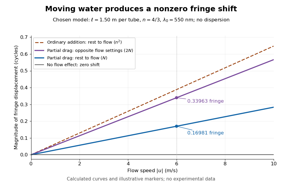
Calculated fringe offsets for chosen parameters: partial drag gives 0.16981 fringe at 6 m/s, whereas equal opposite flows differ by 0.33963 fringe
. Original model curves for tubes of length , refractive index and vacuum wavelength . Solid curves show the first-order rest-to-flow offset and the offset between reversed settings; the dashed curve is the rest-to-flow prediction from ordinary addition of and . No points represent experimental measurements, and optical dispersion is omitted. Details.The Galilean transformation would give phase velocity magnitudes , hence . At the chosen values this is fringe from rest, larger than the special relativity prediction by . A model with no flow-induced change of phase velocity instead gives . The three alternatives are experimentally distinguishable even when is tiny.
Hippolyte Fizeau's positive displacement favoured Augustin-Jean Fresnel's partial-drag law over zero or full drag. He explicitly distinguished support for that law from establishing its underlying luminiferous aether hypothesis.[ref]
The Hypotheses Relating to the Luminous Aether by Hippolyte Fizeau. Comparison of the three predictions and final paragraph qualifying the inference about Fresnel's hypothesis; scanned translation pp. 572–573
The Fizeau experiment therefore supplies a nonzero relative-motion measurement, not a null test proving an luminiferous aether's absence. The derivation above exhibits the same first-order law within special relativity, showing why agreement with the coefficient alone cannot select an physical interpretation.Two limitations matter for precision. The velocity profile sampled by the beam need not equal the cross-sectional average inferred from volumetric flow rate. Also, the Doppler effect gives opposite rest-frame frequencies for the counterpropagating beams. With optical dispersion, the coefficient in the interference fringe formula becomeswhere the refractive index and its derivative are evaluated for stationary water at the laboratory angular frequency . A wavelength-independent therefore defines an approximation, not a precision fit to real water.[ref]
Fizeau’s “Aether-Drag” Experiment in the Undergraduate Laboratory by Thierry Lahaye and others. Section III, p. 499, equation (7), dispersion from opposite Doppler shifts; section IV.B, pp. 499–500, mean flow versus velocity at the beam
Flow reversal removes a fixed phase difference, but a mechanical or temperature change that reverses with the flow can still imitate the signal and must be controlled.Use the schematic below to count the water traversals explicitly. Each stationary tube has laboratory length . In the displayed setting, upper-tube water flows right and lower-tube water flows left, each at speed . Beam A goes right through the upper tube, exchanges tubes at the far optics, and returns left through the lower tube: it follows the flow twice. Beam B goes right through the lower tube and returns left through the upper tube: it opposes the flow twice. Each complete beam path therefore contains total water length , not or . The connecting air paths and fixed optics are assumed to contribute no flow-dependent phase difference.
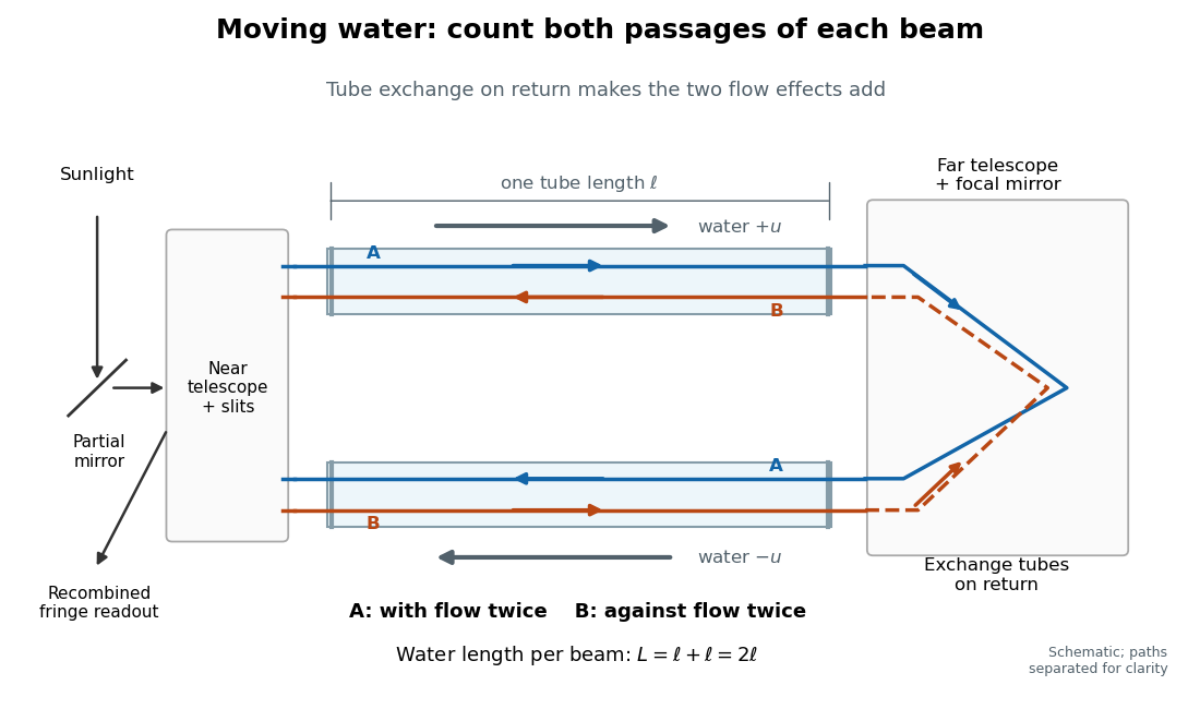
Counterflow path accounting: beam A follows the water in both tubes, beam B opposes it, and each beam traverses total water length 2ℓ
. Original schematic of the tube exchange and recombination, not a scaled optical ray trace. Parallel coloured lines separate overlapping counterpropagating beams for readability. The grey arrows show water flow; reversing both grey arrows exchanges the roles of A and B. Details.Let and be positive phase velocity magnitudes along and against the water flow:For a laboratory source of frequency , where is its vacuum wavelength, define the signed interference fringe offset by the propagation phase difference . This is an equivalent phase delay between steady beams; no stopwatch resolves their transit-time difference. Subtract the zero-flow baseline and expand to first order:Thus one shifted fringe corresponds to one cycle of phase difference. If the stationary pattern has spatial interference fringe spacing , a simple readout model is , where is the interference visibility. The maxima shift by with this choice of screen coordinate. A sign assigned to “rightward” motion depends on the image orientation; the magnitude in fringe units does not.
Reversing both flows gives . The displacement between equal and opposite settings therefore has magnitudeThe factor from comparing opposite flows is additional to the factor already included in . Repeating a round trip in just one flowing tube would instead put a beam with the flow once and against it once; that geometry does not produce the two same-sign contributions drawn here.
The Fresnel drag coefficient is the factor multiplying a transparent medium's velocity in the first-order change of collinear light phase velocity, when optical dispersion is neglected. Here is the medium's refractive index in its rest frame. The name recalls Augustin-Jean Fresnel's partial-drag law; special relativity obtains the same coefficient from the velocity-addition formula without introducing a luminiferous aether.
Let the water move at signed velocity along the positive laboratory axis, with , where is the vacuum speed of light. Assume a transparent medium with constant , uniform flow and negligible optical dispersion. In the water's local rest frame, a collinear constant-phase surface travels at . Dividing the Lorentz transformation differentials along that surface gives the same longitudinal velocity-addition formula as for a particle:The correction comes from the transformed time denominator. Simply adding to would omit it. This argument concerns collinear phase velocity; in a medium with optical dispersion, group velocity is a different quantity.[ref]
Fizeau’s “Aether-Drag” Experiment in the Undergraduate Laboratory by Thierry Lahaye and others. Section III, pp. 498–499, equation (1) and discussion of the collinear wave-four-vector derivation
For , the Fresnel drag coefficient is . A chosen flow speed of therefore changes the forward phase velocity by approximately , even though the stationary-medium phase velocity is about . These are model values. The invariant vacuum speed of light remains ; describes propagation through matter in its own rest frame.
At fixed electric potential difference , a change of capacitance has electrical work input and field-energy increase . The remaining half is mechanical work done by the field, so the force in the direction of increasing overlap is . Equivalently the effective mechanical potential is . For a partially filled coaxial capacitor, this gives , directed inward when . The fringing field of a capacitor supplies the local field gradient and transmits this force even when its small correction to total capacitance is neglected.
Optimal fixed step for quadratic gradient descent by  Codex 0 Created 2026-10-18 Updated 2026-10-31
For a fixed symmetric matrix and positive-definite matrix , what positive step size minimizes the largest coordinate error multiplier over all eigenvector directions? Let and . Since is a convex function of , its maximum over the eigenvalues occurs at an endpoint:Balance the two extremes by solving :Here is the Euclidean norm condition number of . This balance is optimal: for the endpoint exceeds , and for the endpoint exceeds . The optimal worst-case energy factor is , rather than . This optimizes a uniform one-step bound; a particular initial error supported on fewer eigenvectors can have a different best step size.
In the example , , so and . Both eigenvalue directions attain that energy factor, making the displayed history exact. The smaller step size instead givesIts first step reaches , below for , but subsequent progress is limited by the first direction's energy factor . By , the energies are approximately and , respectively; by , the iteration is ahead. A better first step need not yield a faster long-run history.
As the condition number grows, approaches one: stability in the direction of the largest eigenvalue forces small movement along the smallest-eigenvalue direction. This is a precise reason to improve scaling or use a method such as the conjugate gradient method, rather than merely increasing the step size. When , choosing eliminates every error component in one step.
Polarization overlap in interferometric visibility by Codex 0 Created 2026-10-18 Updated 2026-11-05
Codex 0 Created 2026-10-18 Updated 2026-11-05For perfectly temporally coherent beams with unit Jones vectors , their interference term is proportional to the complex inner product . Their interferometric visibility is the displayed expression. Equal beam light intensities reduce it to the magnitude of the polarization overlap. Two linear polarizations at relative angle give ; a linear and a circular polarization give . Perfect coherence does not remove loss of contrast from unequal intensities or orthogonal polarizations.
For an ideal air-gap Fabry–Pérot etalon at normal incidence, the free spectral range is and the peak full width at half maximum is . To separate a pair of lines spaced by by at least peak widths, require . Putting both lines inside one unambiguous free spectral range additionally requires , so . In terms of their vacuum wavelengths, .
The strict order condition needs a margin if tails from adjacent periodic peaks are to be negligible. If every neighbouring peak in a scanned two-line periodic spectrum must be separated by widths, the stronger condition is . Ordinary resolving power alone does not prevent ambiguous repeated orders. A fixed etalon's transmission as a function of wavelength is a periodic-in-frequency filter; it is not automatically a plot of the incident source's spectral lines.
The linear recurrence relation defining the Fibonacci numbers, with and . Its state advances by the matrix , so matrix powers describe repeated updates.
The Barkhausen effect consists of abrupt magnetization changes during a smooth applied magnetic field sweep. Its inductive signal is Barkhausen noise, often arising from collective magnetic domain wall motion.[ref]
The distinction is between a smooth drive and an intermittent material response. A smooth macroscopic hysteresis curve can hide smaller jumps. By Faraday's law of induction, a pickup coil responds to the rate of change of linked magnetic flux, so a rapid jump can be conspicuous even when the total change is small. A pulse is not one chemical atom flipping: neither its height nor the number of audible clicks counts individual electron spins. Qualitative crackling alone does not establish quantum spin; collective switching also admits a classical model with trapped interfaces. Compare the distinct mechanical readout of angular momentum transfer in the Einstein-de Haas effect.
A magnetic domain is a region sharing an ordered magnetic orientation. Different magnetic domains can reduce the total magnetic moment without erasing the local magnetic order. A zero total magnetization therefore does not by itself establish antiferromagnetism.
A ferromagnet is a material that exhibits ferromagnetism. Its magnetic domains can cancel the net magnetization even while each domain remains ordered.
An electron gas confined in one spatial direction, with motion available in the other two. Its electron number per unit area is . The ideal Fermi gas approximation neglects interactions between electrons; an actual two-dimensional electron gas can have important interactions. Confinement alone does not require a magnetic field or Landau levels.
Take two electrical circuits containing coupled inductors. Let their constant self-inductances be , mutual inductance , and positive electrical resistances . Choose current directions so that the off-diagonal entries of the inductance matrix are . Assume a linear, quasistatic model, with no capacitive effects or core hysteresis. The magnetic flux linkages are and . Combining their time derivatives with resistive electric potential differences givesThe secondary is a closed, undriven electrical circuit. Require , making a positive-definite matrix. The chosen current convention fixes the signs; reversing the secondary's reference direction changes the sign assigned to and without changing the physical circuit.
There is an essential switching assumption: the primary loop remains closed when becomes zero. An ideal voltage source then imposes zero electric potential difference, allowing the current to decay. Literally opening an inductive circuit requires additional physics to determine the interruption, including possible capacitance and an electric arc. This closed-return model explains transient induction while keeping that distinction from Faraday's historical making and breaking of contact explicit.
Pinned article: Introduction to the OurBigBook Project
Welcome to the OurBigBook Project! Our goal is to create the perfect publishing platform for STEM subjects, and get university-level students to write the best free STEM tutorials ever.
Everyone is welcome to create an account and play with the site: ourbigbook.com/go/register. We belive that students themselves can write amazing tutorials, but teachers are welcome too. You can write about anything you want, it doesn't have to be STEM or even educational. Silly test content is very welcome and you won't be penalized in any way. Just keep it legal!
Intro to OurBigBook
. Source. We have two killer features:
- topics: topics group articles by different users with the same title, e.g. here is the topic for the "Fundamental Theorem of Calculus" ourbigbook.com/go/topic/fundamental-theorem-of-calculusArticles of different users are sorted by upvote within each article page. This feature is a bit like:
- a Wikipedia where each user can have their own version of each article
- a Q&A website like Stack Overflow, where multiple people can give their views on a given topic, and the best ones are sorted by upvote. Except you don't need to wait for someone to ask first, and any topic goes, no matter how narrow or broad
This feature makes it possible for readers to find better explanations of any topic created by other writers. And it allows writers to create an explanation in a place that readers might actually find it.
Figure 1. Screenshot of the "Derivative" topic page. View it live at: ourbigbook.com/go/topic/derivativeVideo 2. OurBigBook Web topics demo. Source. - local editing: you can store all your personal knowledge base content locally in a plaintext markup format that can be edited locally and published either:This way you can be sure that even if OurBigBook.com were to go down one day (which we have no plans to do as it is quite cheap to host!), your content will still be perfectly readable as a static site.
- to OurBigBook.com to get awesome multi-user features like topics and likes
- as HTML files to a static website, which you can host yourself for free on many external providers like GitHub Pages, and remain in full control

Figure 2. You can publish local OurBigBook lightweight markup files to either OurBigBook.com or as a static website.
Figure 3. Visual Studio Code extension installation.
Figure 5. . You can also edit articles on the Web editor without installing anything locally. Video 3. Edit locally and publish demo. Source. This shows editing OurBigBook Markup and publishing it using the Visual Studio Code extension. 
- Infinitely deep tables of contents:




All our software is open source and hosted at: github.com/ourbigbook/ourbigbook
Further documentation can be found at: docs.ourbigbook.com
Feel free to reach our to us for any help or suggestions: docs.ourbigbook.com/#contact