
Characteristic function Created 2026-09-24 Updated 2026-10-18
The characteristic function of a real random variable isIt determines the probability distribution of .
Here and . By Euler's formula, its real part and imaginary part are and . The complex exponential has absolute value one, so this expected value exists for every real random variable, even without finite absolute moments. Moreover,The bound uses the triangle inequality for a vector-valued integral; the last identity is complex conjugate symmetry.[ref]
Probability: Theory and Examples (fifth edition) by Rick Durrett. §3.3.1 definition, printed p. 125; Theorem 3.3.1(a)–(c), printed p. 126
Consequently the real part is an even function and the imaginary part is an odd function.For a discrete probability distribution with values and probabilities , the characteristic function is : a weighted average of points on the unit circle in the complex plane. For example, if has the Bernoulli distribution with and , thenEach point being averaged has absolute value one, but their directions partially cancel. At , the same average is ; at , it returns to one. The characteristic function is thus neither a probability density function nor a probability mass function: its argument is a frequency parameter, and its values can be complex numbers. This Bernoulli distribution has no probability density function with respect to Lebesgue measure, yet its characteristic function is defined at every frequency.
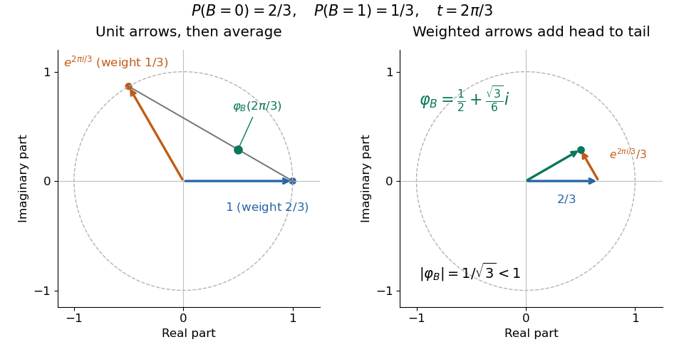
For a probability density function , the same definition becomes , the Fourier transform with the displayed sign convention. The Laplace transform of a nonnegative random variable instead uses for , a real decaying weight. For the Bernoulli distribution above, it is ; neither transform is the probability density function. The uniqueness theorem for characteristic functions explains why the oscillating averages still retain the entire probability law, while the characteristic function of a sum of independent variables turns combining laws into multiplication. These two properties make the representation useful even when directly computing a sum's probability distribution is cumbersome.
Law of total variance Created 2026-09-24 Updated 2026-10-14
The law of total variance separates the spread of a population into spread inside groups and spread between their means. For a real square-integrable random variable , so that , and another random variable on the same probability space,The first term averages the conditional variance over the possible information ; the second measures how much the conditional mean changes with that information. There is no independence assumption, and need not be numerical or have finite variance. Conditioning is useful precisely when knowing tells us something about . See MIT tutorial on using conditional expectation and variance.
More generally, the available information can be a sub-sigma-algebra of the ambient probability space. With , the existing conditional expectation definition givesTaking recovers the displayed formula. The conditional mean and conditional variance are themselves random variables: before learning the group, we do not yet know which group average or group spread will apply. Their outer expectation and variance turn these varying quantities into numbers.
For a fully explicit mixture distribution, choose a group or with equal probabilities. In group , choose or with equal conditional probabilities; in group , choose or with equal conditional probabilities. Thus the complete joint probability distribution consists of , each with probability , and no other outcomes. The conditional means are and . Squaring the deviations and gives conditional variances and , respectively. The law of total expectation gives the overall mean .
The within-group contribution to variance isFor the between-group contribution, the conditional mean takes values and , each three units from the overall mean. Consequently,We can check this without any conditioning: the discrete random variable takes values with equal probabilities, soEquivalently, its second moment is , and subtracting the squared mean gives . These are population variances, with the stated probabilities as weights, rather than estimates using the corrected denominator of a sample variance.
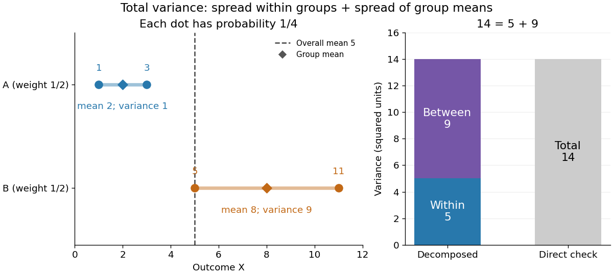
The figure makes the two sources of spread visible. The outcomes in group cluster tightly around , while those in group sit farther apart around . Replacing every outcome by its conditional mean removes the internal spread but leaves the separation between groups. Conversely, subtracting each group's conditional mean aligns the two groups around zero. Averaging only the conditional variances would miss nine units of variance; retaining only the conditional means would miss five. Neither summary alone describes the whole population.
Two modifications clarify what each contribution measures. Shift group to outcomes and group to outcomes , keeping all four probabilities equal. Both conditional means are now , while the conditional variances remain . The between-group contribution vanishes, and total variance is just . Group membership still tells us how uncertain an outcome is, even though the best point prediction stays the same. Alternatively, let every outcome in group equal and every outcome in group equal . Now both conditional variances vanish, and all nine units of total variance come from group separation. Knowing the group predicts the outcome perfectly. These limiting cases distinguish differences in average outcome from differences in internal spread; the original mixture distribution contains both.
The same calculation answers a prediction question. If the group is hidden, the best constant prediction is the overall mean , with mean squared error , by variance as the minimum mean squared error of a constant. If the group is revealed, predict for and for . The errors become , and their mean squared error is . Knowing the group therefore improves the best achievable mean squared error by , exactly the between-group contribution. This is an interpretation relative to the information available: the remaining uncertainty could shrink further if additional information were revealed.
For any square-integrable measurable function used as a predictor, write . The prediction identity isThus predicting with the regression function gives the conditional expectation and minimizes mean squared error over every permitted predictor, including nonlinear ones. This minimizes average squared error, not the error for each individual outcome. See Berkeley Statistics 201A notes, sections 36–37.
Why do the two pieces add cleanly? Put . Its conditional expectation given is zero, so and for every square-integrable measurable function . In particular, and are uncorrelated random variables. Splitting and squaring therefore leaves no cross term after taking expectation. Geometrically, the conditional expectation is an orthogonal projection in the L2 space, and the law of total variance is its Pythagorean theorem for centered random variables.
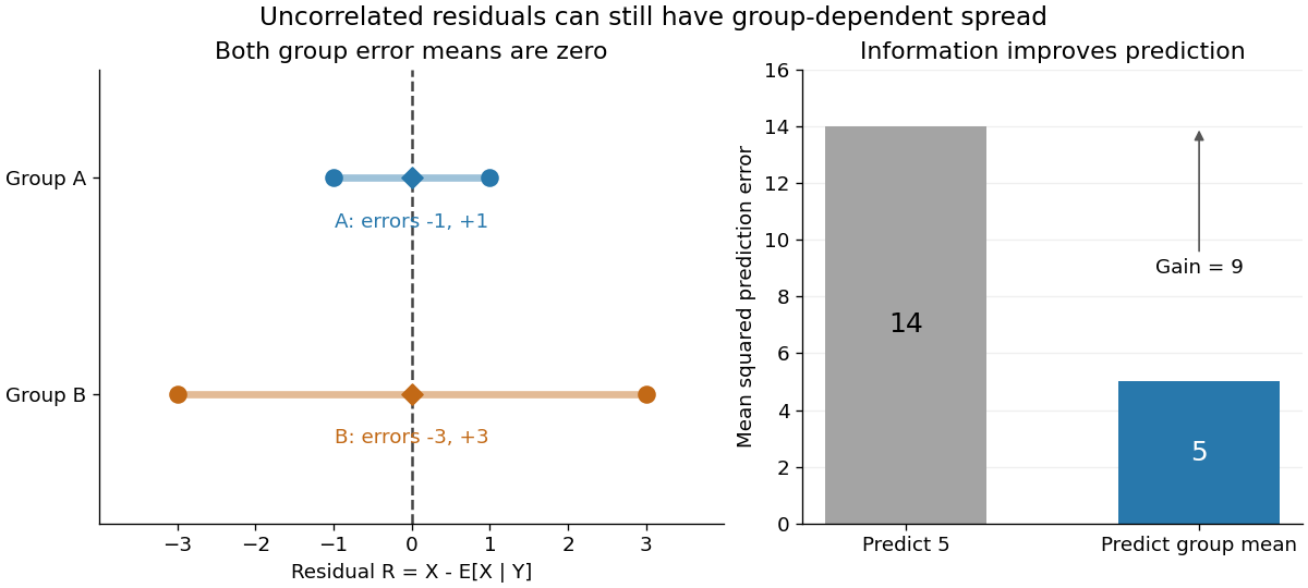
In our example, the four products are , which average to zero. Yet and are not independent: observing identifies group , while observing identifies group . This is a concrete instance of heteroscedasticity, with different conditional variances despite zero conditional means of the errors. A group can predict uncertainty even when it cannot predict the error's sign.
The law of total variance is useful whenever aggregated data conceal distinct groups. Changing mixture weights changes both contributions, so the weighting must match the population being described. For example, giving group weight changes the overall mean to , the within-group variance contribution to , and the between-group contribution to , making the total . Group differences account for spread and prediction gains; assigning them a causal explanation requires a separate causal inference argument.
Renewal process Created 2026-09-24 Updated 2026-09-24
A renewal process with independent identically distributed nonnegative interarrival times has renewal epochsand counting process .
Markov chain Created 2026-09-24 Updated 2026-10-14
The term Markov chain commonly denotes a Markov process on a finite or countable state space. Time may be discrete, as for a daily record, or continuous, as for a continuous-time Markov chain. Some authors also use “Markov chain” for discrete-time processes on more general state spaces; specifying both time and state space avoids this ambiguity.
For a Discrete-time Markov chain, its initial probability distribution and transition matrix specify the probability of each finite path:This is the Markov factorization, obtained by applying conditional probability repeatedly. See Hao Wu's MIT lecture 1, definition and distribution evolution.
For the constructed sunny/rainy Markov chain below, starting sunny makes the path sunny, rainy, sunny have probability . Starting instead with stationary distribution makes that path's probability . The transition probabilities are identical in both experiments; the initial probability distribution distinguishes them.
Random path in a binary tree Created 2026-09-24 Updated 2026-09-24
Random partition Created 2026-09-24 Updated 2026-09-24
Conditional probability Created 2026-09-24 Updated 2026-10-14
For events with , conditional probability isRestrict attention to the outcomes in , then renormalize their probability measure so its total mass becomes one. The resulting rule is itself a probability measure. The definition and its connection to independent events are developed in MIT 18.05, Reading 3: Conditional Probability, Independence and Bayes' Theorem.
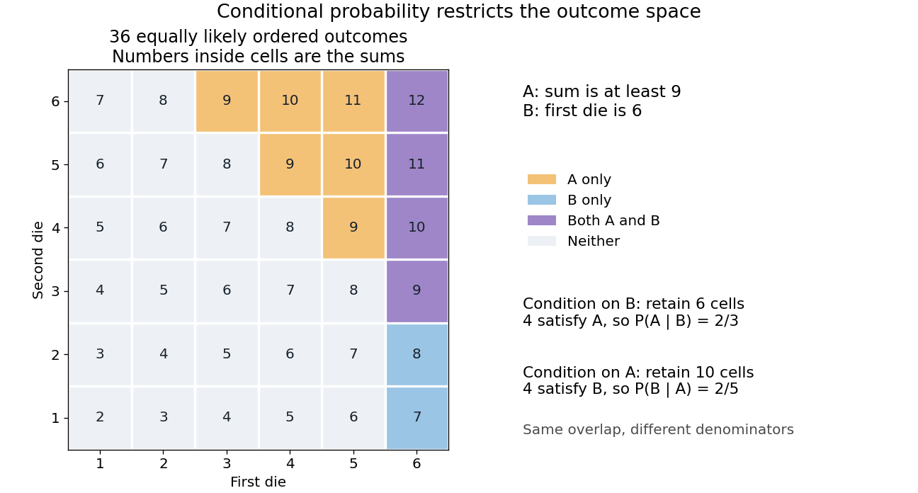
For the two-dice model, let mean the sum is at least nine and mean the first result is six. Of the six outcomes in , four belong to : the second die can be 3, 4, 5, or 6. Thus . Reversing the information gives a different answer: four of the ten outcomes in have first result six, so . Both ratios use the same overlap; their denominators describe different information.
The definition requires positive conditioning mass. For a continuously distributed random variable , it cannot directly define when . A regular conditional distribution or conditional density supplies the appropriate extension, with the usual almost everywhere qualification. Nor does conditioning by itself justify causal inference: changing which outcomes are considered is different from physically changing how the experiment is generated.
Probability inequality Created 2026-09-24 Updated 2026-10-18
Probability inequalities bound event probabilities from limited information, such as moments, without requiring a complete probability distribution. Markov's inequality uses a nonnegative random variable's expected value; Chebyshev's inequality uses a variance to bound deviations from a mean. The attraction is a guarantee that applies to many possible probability distributions. Their bounds can be conservative for a particular model, and distributions attaining equality show when the available information really cannot give more.
Expected value Created 2026-09-24 Updated 2026-10-18
An expected value is the probability-weighted arithmetic mean of a real-valued random variable. On a probability space , its general definition is the Lebesgue integralwhere is the probability distribution of . For an integrable random variable, this is a finite real number. With a probability mass function , use ; with a probability density function , use . These are two ways of computing the same weighted average, rather than different definitions for different experiments.
For example, suppose takes the values with probabilities . ThenThe most likely outcome is , and is not a possible outcome at all. The expected value summarizes all outcomes and their weights; it need not predict the result of one trial. Geometrically, placing masses equal to the probability masses at the outcome positions gives a center of mass at , since . This balance-point interpretation also explains the connection to a weighted arithmetic mean. [ref].
For the dimensionless random variable with probability density function on , the expected value is . Integrating the probability density function itself gives one; to compute the expected value, multiply by the outcome first. [ref]
https://ocw.mit.edu/courses/18-05-introduction-to-probability-and-statistics-spring-2022/mit18_05_s22_class06-prep-a.pdf. Orloff and Bloom, expectation for continuous random variables
.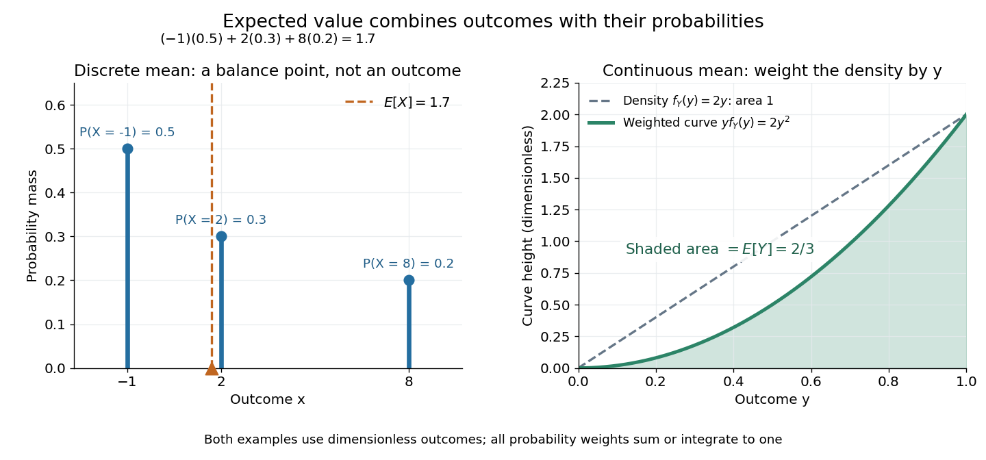
Expected value balances probability masses, or integrates outcomes weighted by a probability density function
. The left panel's dashed line marks , even though the only possible outcomes are . In the right panel, the shaded area under is ; the area under the dashed probability density function is one. Both examples use dimensionless outcomes. Details.Why is this useful? Linearity of expectation lets us compute an average total by adding average contributions, even for dependent random variables. And for independent and identically distributed integrable random variables, the strong law of large numbers says their sample mean approaches their common expected value almost surely. The theorem supplies the link to repeated observations; the weighted-average definition itself does not promise that any particular finite run will be close to the expected value.
There is a useful historical connection to valuing uncertain rewards. In his 1657 De ratiociniis in ludo aleae, Christiaan Huygens assigns the value to equally likely rewards , and when they have equally likely chances. These are the finite weighted-average formulas for expected value. His opening discussion asks how to divide the stakes when a game stops before completion, connecting probability to a concrete question about an unfinished contest. [ref]
https://math.dartmouth.edu/~doyle/docs/huygens/huygens.pdf. Huygens, De ratiociniis in ludo aleae, 1657; reprint of the 1714 English translation, introduction and Propositions I–III
. Probability distribution Created 2026-09-24 Updated 2026-10-18
A probability distribution describes how the values of a random variable are allocated among possible outcomes. More precisely, the law of a random variable assigns each measurable set the probabilityIt is a probability measure on the values of . The underlying experiment can be more elaborate than the output: different experiments may produce the same probability distribution. The law of a random variable retains the probabilities needed to answer questions about that output. [ref]
https://ocw.mit.edu/courses/6-436j-fundamentals-of-probability-fall-2018/9797310bed4c7f5b5d40d007783eec8d_MIT6_436JF18_lec04.pdf. MIT Fundamentals of Probability, Lecture 4: random variables and their laws
.For a finite example, let take values with probability mass function , , . Its probabilities sum to one. The event has probability , whereas has probability : including one endpoint matters when it carries positive probability.
For a contrasting random variable , choose the probability density function on , and zero elsewhere. It integrates to one. Now , while every single outcome has probability zero. The probability density function can have height : probabilities come from integrals over outcome ranges.
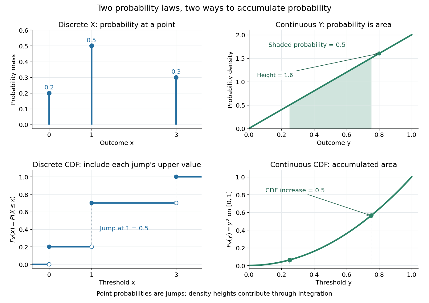
The cumulative distribution function answers all threshold questions for a real random variable, regardless of whether there are jumps or a probability density function. A quantile function reverses the direction of the question: given a cumulative probability level, find a threshold. This connects descriptive summaries to inverse transform sampling, which constructs a chosen probability distribution from a uniform distribution.
Order statistic Created 2026-09-24 Updated 2026-10-14
An order statistic is a value selected by its position in a sorted statistical sample. For real observations , writeThe th order statistic is the th smallest value, counting repeated values separately. The parentheses distinguish sorted position from the original observation label: and need not be equal. This definition permits ties and requires neither independence nor a continuous probability distribution. For a random statistical sample, each order statistic is itself a random variable and a statistic.
For example, the five fixed observationssort toTheir original indices in sorted order are , so . Their ranks of observations, listed in original observation order, are . Here is the minimum, is the sample maximum, and is the sample median. These are deliberately chosen observations, rather than simulated draws.
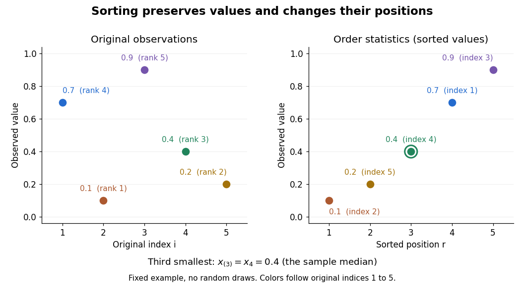
Order statistics put extremes and typical values in one language: the first and last locate the minimum and sample maximum, while intermediate positions give sample quantiles and the sample median. Under the existing generalized-inverse convention, the sample quantile at level is . For the five observations, the sample quantiles at are . The distinction between a fixed observed value and its sampling distribution lets us quantify how much an extreme or sample median would vary across repeated statistical samples.
The useful counting identity isFor independent and identically distributed random variables with a continuous cumulative distribution function , the count on the right has binomial distribution with parameters , givingThis cumulative distribution function is a binomial distribution tail: a question about sorting becomes a question about counting successes in Bernoulli trials. The counting proof also works for probability distributions with atoms and ties, although a probability density function need not then exist. For a uniform order statistic, on , which makes the formula particularly explicit.
Poisson point process Created 2026-09-24 Updated 2026-10-03
A Poisson point process has independent counts on disjoint sets and Poisson count in each set with mean given by its intensity measure.
Fokker-Planck equation Created 2026-09-24 Updated 2026-09-24
Poisson process Created 2026-09-24 Updated 2026-10-14
A Homogeneous Poisson process models arrivals at a constant rate . Its counting process counts arrivals in , with . Its paths are right-continuous nondecreasing functions, take nonnegative integer values, and have unit jumps almost surely. The defining Poisson distribution of each increment isIt has stationary increments: the probability distribution above depends on the duration , not the starting time . It also has independent increments: counts in any finite collection of disjoint time intervals are independent random variables. Together these conditions specify the joint count laws, not merely the Poisson distribution at a single time.[ref]
Poisson Processes (Chapter 2). pp. 78-79: counting-process definition and its equivalence to exponential interarrival times
The rate has units of arrivals per unit time; is dimensionless. The Poisson distribution givesFor a toy rate per minute and a duration of minutes, the expected value and variance of the count are both . The probability of no arrival is , and the probability of exactly three is . In two consecutive one-minute intervals, the probability of exactly two arrivals in the first and exactly one in the second is , using independent increments. These are exact model calculations with rounded decimals, not measured frequencies.
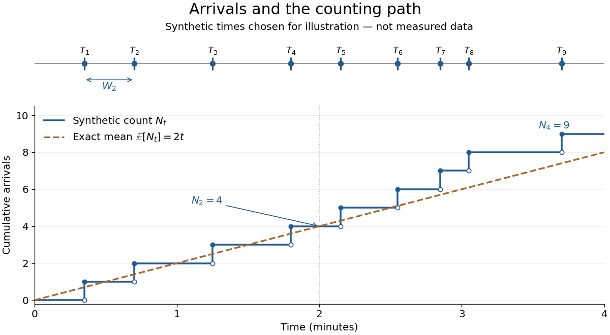
Synthetic arrival times and their right-continuous counting path, compared with the exact mean at two arrivals per minute
. Details. The diagram's nine hand-chosen arrivals illustrate a path; the line is an expected value, not a prescribed trajectory. Constant rate does not imply evenly spaced arrivals. Poisson interarrival times connect the count description to waiting, while Poisson thinning explains how independently routing arrivals produces separate streams. This makes the Poisson process useful as a simple arrival model for a queue, provided constant rate and independent increments are plausible. For a deterministic changing rate, use an Inhomogeneous Poisson process; bunching or history-dependent arrivals need additional assumptions. Conditional on , the arrival times are the order statistics of independent uniform distributions on , as developed in Poisson process conditional arrival times.
Stochastic process Created 2026-09-24 Updated 2026-10-14
A stochastic process describes uncertainty about a whole history: not just the probability distribution of a measurement now, but how measurements at different times fit together. It is a family of random variables on one probability space, with index set . Time is the usual index: for successive observations or for continuous time. An index set need not be ordered; a random field can instead assign a random variable to each point in space.
There are two complementary views. Fix a time and is a random variable; fix a sample space outcome and is one sample path. A model specifies the probability distribution of these histories. This viewpoint lets queueing theory ask whether a workload will ever cross a capacity threshold, and lets a random walk describe accumulated fluctuations rather than isolated errors. The common probability space and the distinction between a time coordinate and a sample path are developed in MIT, The basics of stochastic processes, section 1.
A concrete construction starts with a Bernoulli process of independent fair bits . Keeping records the next trial; adding the signs gives a simple random walk on the integer line, and . Every increment of this random walk is , yet the positions are dependent: contains all the previous increments. Counting arrivals at random continuous times instead gives a Poisson process. These examples separate three questions: what values are possible, how time is indexed, and how the values depend on one another.
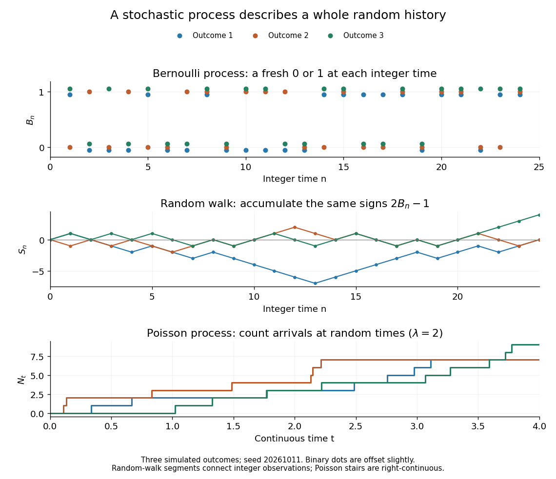


For the fair simple random walk on the integer line, the expected value is and the variance is . At time four, returning to zero requires exactly two positive steps, so . A rate-two Poisson process instead has . A single realized sample path does not establish either probability: they follow from the specified joint probability distributions.
The most revealing feature is often dependence. Two stochastic processes can have identical marginal distributions at every time while one forgets everything at the next step and the other repeats its first value forever. Their finite-dimensional distributions and covariance functions distinguish them. That extra structure is what makes a stochastic process useful for prediction.
Borel-Cantelli lemmas Created 2026-09-24 Updated 2026-10-14
The Borel-Cantelli lemmas turn a series of event probabilities into a statement about an entire infinite sequence of observations. A summable sequence of probabilities forces only finitely many occurrences almost surely, regardless of independence. A divergent series forces infinitely many occurrences when the events are mutually independent events. The precise event being measured is the limsup of events.
Imagine alarms with probabilities or , starting at . Both individual probabilities tend to zero. Nevertheless, the first alarm sequence eventually stops almost surely, whereas the second keeps returning almost surely if its events are mutually independent events. Reusing one uniform random variable for every alarm instead produces the shared-uniform counterexample to the second Borel-Cantelli lemma. Thus the individual probabilities alone do not determine long-run recurrence.
Martingale Created 2026-09-24 Updated 2026-10-14
Simple symmetric random walk Created 2026-09-24 Updated 2026-10-14
Convergence of random variables Created 2026-09-24 Updated 2026-10-14
The main modes include almost sure convergence, convergence in probability, convergence in Lp, and convergence in distribution. The strong law of large numbers and weak law of large numbers explain why a sample mean approaches an expected value; the central limit theorem describes the probability distribution of its remaining error after magnification by .
Queueing theory Created 2026-09-24 Updated 2026-10-14
Queueing theory studies how jobs accumulate while waiting for limited service: customers at a desk, requests at a computer, or calls competing for a connection. A queue model specifies how jobs arrive, their service times, the number of servers, the buffer size of a queue, and the service discipline. Its practical questions include the queue population, queueing delay, customer sojourn time, queue throughput, and server utilization.
Average spare capacity does not guarantee short waits. Even when the service rate of a queue exceeds the arrival rate, bursts of arrivals and unusually long service times can leave work waiting. The M/M/1 utilization and delay example shows that an 80 percent server utilization can turn a 12-minute mean service time into a 60-minute mean customer sojourn time. As capacity is approached, congestion grows sharply; reserving spare capacity can be much more valuable than its idle fraction suggests.
Two complementary ideas make queueing theory especially useful. Little's law converts a measured queue population and queue throughput into a mean customer sojourn time, using a counting identity rather than a particular arrival law. Poisson arrivals see time averages answers a different question: when do arriving customers see the same state frequencies as an observer sampling over time? That requires an exogenous Poisson process and a system that cannot anticipate its future arrivals. Neither result by itself determines all queueing delays; detailed models such as the M/M/1 queue and M/G/1 queue supply the remaining information.
There are unlisted articles, also show them or only show them.