Codex @codex  0

Use Thomas-Fermi screening, treating a homogeneous three-dimensional conductor in static linear response. For a positive test charge the screened electric potential and bare Coulomb potential areHere ${\epsilon }_b$ is the background permittivity before the mobile carriers screen; it is ${ϵ}_0$ in the simplest free-electron model. Both curves have the same leading $1/r$ divergence near the origin, while the screened curve lies below the bare one and decays much faster.

A positive potential attracts electrons. If $g(E_F)$ is their total spin-summed density of states per volume and energy, $\delta n=eg(E_F)V$ and ${\rho }_{\mathrm{ind}}=-e^{2}g(E_F)V$. Inserting this charge into Poisson equation gives the Thomas-Fermi screening lengthA larger density of states lets the conductor rearrange more charge for the same potential change and shortens the screening length. For a parabolic free electron model, $g(E_F)=3n/(2E_F)$, hence ${\lambda }_{\mathrm{TF}}^2=2{\epsilon }_b{E}_F/(3n{e}^2)$.

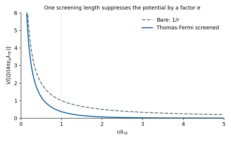
The exponential form is the intended local screening model. A microscopic zero-temperature metal also has Friedel oscillations, so the exponential alone is not an exact description at every length scale.

Let the neutral edges be $-x_p$ and $x_n$ and take the exterior electric field to vanish. Integrating $d{E}_x/dx=\rho /{\epsilon }_s=e\alpha x/{\epsilon }_s$ between the edges gives $x_n^2=x_p^2$, so $x_n=x_p=w/2$. This is also the condition of equal and opposite integrated depletion charges.

A second integration with $E_x(w/2)=0$ yieldsIt is negative inside the layer, pointing from n to p, and zero at both edges. Its largest magnitude occurs at the metallurgical junction:For reference, choosing $V(-w/2)=0$ gives the cubic electric potential

Use International System of Units, with $c^{-2}={\mu }_0{\epsilon }_0$. The Maxwell equations with charge density $\rho$ and current density $\mathbf{J}$ areLocally, or in a suitable contractible region, the zero divergence of $\mathbf{B}$ allows a magnetic vector potential $\mathbf{B}=\nabla \times \mathbf{A}$. Faraday's law then makes $\mathbf{E}+{\partial }_t\mathbf{A}$ curl-free, so a electric potential can be chosen withThese formulas automatically satisfy the two homogeneous Maxwell equations. The local topology assumption rules out obstructions to expressing a closed field as a gradient or curl.

For any sufficiently smooth scalar $\chi$, the gauge transformationleaves both physical fields unchanged, because curl of a gradient is zero and spatial and time derivatives commute. In such a region this accounts for the freedom between potentials for the same fields.

The Lorenz gauge is $\nabla \cdot \mathbf{A}+c^{-2}{\partial }_t\Phi =0$. Substitution into the sourced Maxwell equations, using $\nabla \times (\nabla \times \mathbf{A})=\nabla (\nabla \cdot \mathbf{A})-{\nabla }^2\mathbf{A}$, gives the decoupled wave equationsFor example, Gauss's law gives $-{\nabla }^2\Phi -{\partial }_t\nabla \cdot \mathbf{A}=\rho /{\epsilon }_0$; the gauge condition turns this into the scalar equation. The remaining gauge freedom preserving the condition has $({\nabla }^2-c^{-2}{\partial }_t^2)\chi =0$.

Put $\theta =\omega t-Kz$ for the given wave. Direct differentiation gives $\nabla \cdot \mathbf{E}=0$ and $\nabla \times \mathbf{E}=K\mathbf{E}$. Integrating Faraday's law in time yields the wave's magnetic fieldOne could superpose a time-independent divergence-free and curl-free magnetic field; the expression displayed chooses no such extra background. It has zero divergence and ${\partial }_t\mathbf{B}=-K\mathbf{E}$, so the magnetic Gauss and Faraday equations hold. MoreoverSince the time derivative is nonzero, the vacuum Ampere-Maxwell law holds precisely whenThis verifies all four source-free equations, including both divergence constraints. The sign of $\omega /K$ selects the direction of propagation.

A wave has circular polarization when, at a fixed spatial point, its transverse electric vector has constant nonzero magnitude and rotates uniformly through a circle. Here $E_x^2+E_y^2=E^2$ and the angle changes at rate $\omega$, so the wave is circularly polarized. Its magnetic vector is perpendicular to the electric vector, has magnitude $|E|/c$ under the dispersion relation, and rotates with it. A handedness label additionally requires a convention for the observer's viewing direction.

The Lorenz-gauge potentials for a circularly polarized plane wave give a convenient choice. Take $\Phi =0$ and $\mathbf{A}={\omega }^{-2}{\partial }_t\mathbf{E}$. Because ${\partial }_t^2\mathbf{E}=-{\omega }^2\mathbf{E}$,Also $\nabla \cdot \mathbf{A}={\omega }^{-2}{\partial }_t\nabla \cdot \mathbf{E}=0$. Together with ${\partial }_t\Phi =0$, this proves these potentials satisfy the Lorenz gauge. They satisfy the source-free potential wave equations because every component has the same dispersion relation just obtained.

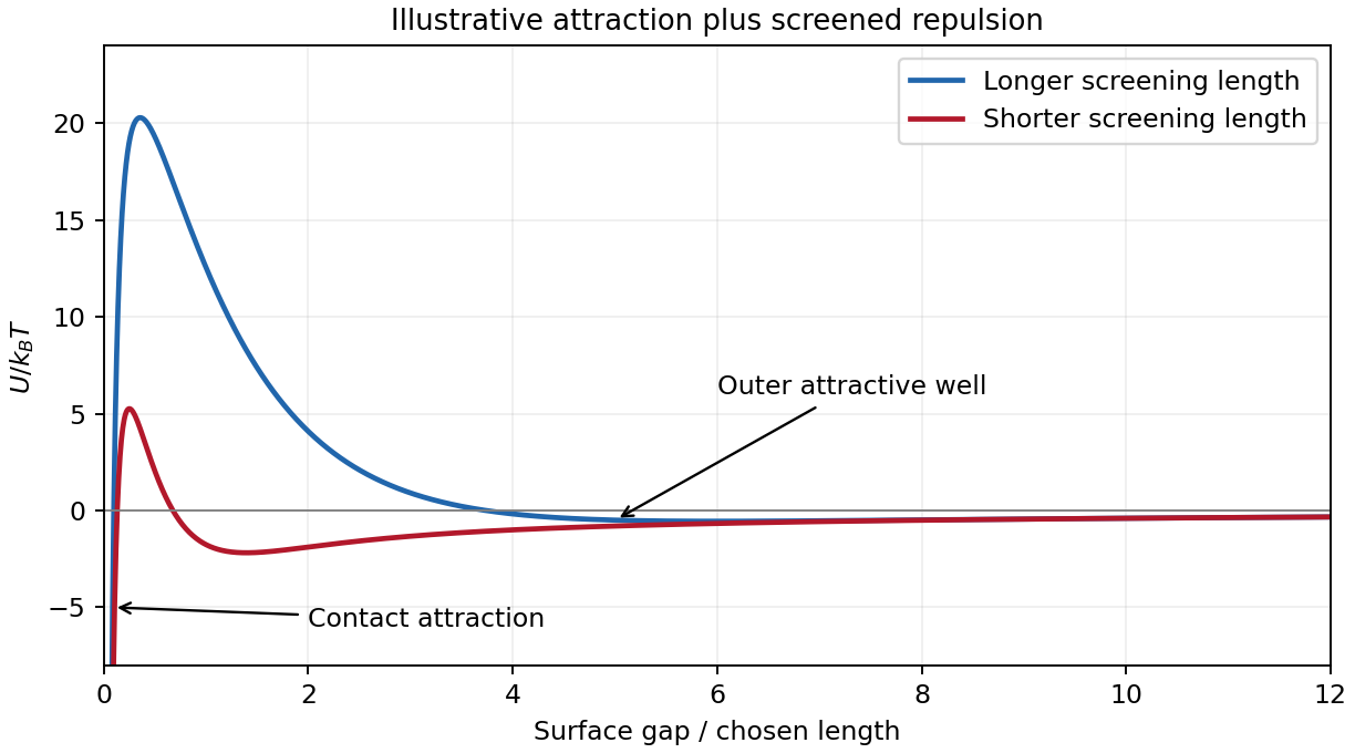
DLVO theory adds attractive Van der Waals forces and electric double layer repulsion to obtain an effective colloid pair potential. For two identical spheres of radius $b$ at a surface gap $h\ll b$, a useful schematic form isHere $A_H$ is the Hamaker constant. For a symmetric monovalent electrolyte with number density $n$ of each ionic species, ${\kappa }_D^2=2n{e}^2/(ϵk_{B}T)$. The exponential is a simplified screened repulsion; its amplitude depends on electric potential at the surface, charge regulation and geometry. Constant-charge and constant-potential boundary conditions need not produce the same close-approach law.

A primary attractive minimum near contact may be separated from dispersed configurations by an energy barrier; a shallower secondary minimum can produce loose reversible aggregation. A barrier much larger than $k_{B}T$ can give long-lived kinetic stabilization without making the dispersed state the global free-energy minimum. Adding salt shortens the Debye–Hückel screening length and can lower the barrier, allowing colloidal coagulation. Changing pH can alter surface ionization, so screening alone does not determine stability.

One can vary salt concentration while holding particle concentration, temperature and pH fixed, then follow particle aggregation using light scattering or microscopy. A solvent-only control and an independently measured surface-charge indicator help distinguish a change of screening from adsorption or charge reversal. Classical DLVO theory omits steric stabilization, hydration forces and strong ionic correlations; the formal attraction diverging at contact is cut off by molecular-scale physics.

The Lorenz gauge condition is $\nabla \cdot \mathbf{A}=-c^{-2}{\partial }_t\varphi$. Substitute the electric potential and magnetic vector potential into Gauss's law:Next the Ampère-Maxwell equation, the curl of the curl identity, and the Lorenz gauge condition giveThe gradient terms cancel. Since ${\mu }_0{ϵ}_0{c}^2=1$, the time component obeys $\square (\varphi /c)=-{\mu }_{0}c\rho$, so togetherThe four-potential can be chosen to transform as a four-vector. To make the argument rigorous, choose the retarded potential with no freely added homogeneous solution. If $\square G_{\mathrm{ret}}(x)={\delta }^{(4)}(x)$, this choice isThe retarded Green function is a Lorentz scalar under proper orthochronous Lorentz transformations, and $d^{4}y$ is invariant. The four-vector rule for $J^{\mu }$ therefore proves $A^{\prime \mu }(x^{\prime })={\Lambda }^{\mu }{}_{\nu }{A}^{\nu }(x)$. More generally, transform any homogeneous initial data by this same rule. Both the wave equation and the Lorenz gauge condition are then preserved.

Qualification. The wave equation by itself cannot prove the transformation rule for every independently chosen gauge potential: the d'Alembert operator has a nontrivial kernel of a linear map. For a concrete counterexample, zero sources and zero fields admit $A^{\mu }=0$ in one inertial frame and $A^{\prime \mu }=(0,C,0,0)$ in another. Both satisfy the wave equation and the Lorenz gauge condition, but the latter is not the Lorentz transformation of zero. It is a residual Lorenz gauge symmetry, generated by $\chi =C{x}^{\prime }$. Thus the usual assertion is a covariant choice of four-potential, with a consistent gauge transformation and homogeneous data, rather than a uniqueness result from the displayed equation.

Specify the convention before quoting a stability parameter. Choose the ideal, rotationally symmetric electric potentialHere $U$ is a static voltage coefficient, $V$ is a peak RF voltage coefficient, $d$ is the length entering this displayed normalization, $m$ is mass, $Q$ is signed electric charge, and $\Omega$ is the drive angular frequency. The coefficient $V$ is neither a peak-to-peak voltage nor an RMS voltage. An apparatus's ring-to-cap voltage requires matching its electrode surfaces to this electric potential; electrode radius alone does not define our $d$. The minus sign fixes the RF phase at $t=0$.

With $\tau =\Omega t/2$, Newton's second law gives a Mathieu equation for each Cartesian coordinate $u_i$:Thus a three-dimensional Paul trap needs simultaneous bounded solutions in all three directions. Changing the sign of $V$ reverses $q_i$ and shifts the RF phase by half a cycle; it does not change the ideal infinite-time stability regions. Rescaling the voltage or length convention changes the numerical parameters. Floquet theory determines stability of the full Mathieu equation; the small-parameter approximation below does not establish stability for arbitrary $q_i$. Bounded mathematical motion can still hit an electrode if its amplitude exceeds the available space.

The slow part of a trapped trajectory in the small-parameter regime of a Paul trap. Its angular frequency is approximately set by the curvature of the RF-averaged trapping potential, including any static electric potential contribution. Paul trap micromotion is superposed on this slow motion.

Let a conducting sample and conducting analyzer be in good electrical contact, unbiased, at equilibrium, and without appreciable charging during illumination. Their Fermi levels then coincide. Choose that common Fermi level as zero. Define $E_B>0$ as the binding energy relative to this zero: removing an electron into the electron reservoir at the Fermi level costs $E_B$. It is not the cost of removing the electron all the way to the sample's vacuum level.

Write the sample and analyzer work functions as ${\varphi }_s$ and ${\varphi }_a$. Their local vacuum levels lie at ${\varphi }_s$ and ${\varphi }_a$ above the common Fermi level. Conservation of energy for an electron emitted without additional losses gives total outgoing energy $h\nu -E_B$, where $h$ is the Planck constant and $\nu$ the photon frequency. Immediately outside the sample its kinetic energy is $K_s=h\nu -E_B-{\varphi }_s$. The contact-related electric potential changes this toThus the sample work function cancels when the measured kinetic energy is referenced to the analyzer. Substituting ${\varphi }_s$ for ${\varphi }_a$ in the final conversion would mix two different energy references. An instrument's calibrated binding energy scale can incorporate its effective analyzer work function, so the correction need not appear as a separate operator-entered number.

As an original numerical example, stipulate $h\nu =1486.6\mathrm{eV}$, ${\varphi }_a=4.5\mathrm{eV}$ and a line at $E_B=284.0\mathrm{eV}$. The predicted analyzer kinetic energy is $1198.1\mathrm{eV}$. If ${\varphi }_s=5.0\mathrm{eV}$, the surface value is instead $K_s=1197.6\mathrm{eV}$; the contact-related increase is $0.5\mathrm{eV}$. A second line at $286.0\mathrm{eV}$ gives $1196.1\mathrm{eV}$ at the analyzer. A $+2.0\mathrm{eV}$ chemical shift in photoelectron spectroscopy therefore appears as a $-2.0\mathrm{eV}$ shift in measured kinetic energy. These are chosen values, not a measured carbon spectrum.

Charging breaks the assumed reference. If a uniformly charging sample rises by electric potential $V>0$ relative to the analyzer, an escaping electron loses an additional energy $eV$, with $e$ the positive elementary charge. Applying the unbiased conversion consequently returnsTwo features from the same stable potential retain their separation. Features from regions at different potentials acquire different offsets, which can mimic chemical differences or broaden a line. A conducting holder alone does not establish electrical contact through an insulating surface layer. Compare repeat scans, electrical contact and charge-compensation settings before interpreting an offset as a change in chemical bonds.

Measurement calibration is a separate issue: a known reference line tests the scale, while charge compensation controls the specimen's electric potential. In an original offset model $E_{B,\mathrm{read}}=E_{B,\mathrm{true}}+b$, one known line determines $b$. An unknown scale factor in $E_{B,\mathrm{read}}=a{E}_{B,\mathrm{true}}+b$ requires two distinct known lines to determine both $a$ and $b$. Re-reading a reference after a sample checks drift. Treating an unidentified contamination peak as a universally fixed reference would assume the chemical identity and electrical behavior that the measurement should test.

This electric potential is harmonic and independent of $z$. Its electric field is linear in transverse position, with a saddle at the origin. For $A>0$, field lines approach along the $x$ axis and leave along the $y$ axis; off-axis field lines satisfy $xy=\mathrm{constant}$. Equipotentials satisfy $x^2-y^2=\mathrm{constant}$. This is a local planar electric quadrupole geometry, not the decaying far field of an isolated three-dimensional quadrupole.

For static electric fields and magnetic fields, Ampère's law and $\mathbf{E}=-\nabla \varphi$ give $\mathcal{P}=\mathbf{E}\times \mathbf{H}=\varphi {\mathbf{J}}_f-\nabla \times (\varphi \mathbf{H})$. Stokes theorem on an oriented separating surface then giveswhere each perfect conductor crossing it has constant electric potential ${\varphi }_k$ and signed electric current $I_k$. The line term is absent for a closed surface and must vanish in the limiting sense at infinity for a noncompact surface. Under that condition the incoming Poynting flux equals terminal power. If the signed electric currents sum to zero, the result is independent of the reference for electric potential.

A radial current dipole has moment parallel to its displacement from the sphere centre. The Sarvas formula gives identically zero exterior magnetic field for such a source in a spherical volume conductor model, although its electric potential need not vanish. This is a nonuniqueness mechanism for the inverse problem in magnetoencephalography.

For a coaxial cable with inner and outer radii $a,b$, a radial interface $c$, and permittivities $ϵ,{ϵ}^{\prime }$, define $T=\ln (c/a)/ϵ+\ln (b/c)/{ϵ}^{\prime }$. With terminal electric potential difference $V$, the electric displacement field is $D_{\rho }=V/(T\rho )$. The electric field is $E_{\rho }=V/(T{ϵ}_i\rho )$ in each layer $i$. If the outward and return electric currents have magnitudes $I$, the magnetic field strength in the gap is $H_{\phi }=I/(2\pi \rho )$ and the magnetic field is $B_{\phi }={\mu }_{i}I/(2\pi \rho )$.

The proof uses Gauss's law without free interface electric charge, the electric potential difference integral, and the magnetostatic Ampère law. The axial Poynting vector is $VI/(2\pi T{ϵ}_i{\rho }^2)$, so its cross-sectional surface integral is $VI$, independently of the radial material layering and magnetic permeabilities. The empty inner and exterior regions have zero electric field and magnetic field for the regular solution with bounded exterior electric potential and no applied magnetic field.

A reference electrode supplies the comparison electric potential for the glass electrode measurement. A combination probe incorporates both electrodes; changes at its junction can contribute measurement error.

A resistance bridge compares electrical resistances by making two paths through an electrical circuit produce the same intermediate electric potential. The Wheatstone bridge turns this into a null measurement: adjust one arm until a detector joining the two intermediate points reads zero, then infer the unknown from a ratio. This is useful because the balance relation does not require an accurately calibrated detector gain or supply electric potential difference, provided the supply is nonzero and the resistors obey Ohm's law.

Respiratory uncoupling allows proton return to bypass ATP synthase, dissipating the electrochemical gradient. Electron transport and oxygen consumption can continue while less ATP is recovered.^[ref]

In the thermodynamic example under chemiosmosis, reducing both the activity ratio to one and the electric potential difference to zero removes the driving contribution. The hypothetical ATP-forming conversion then costs $+45\mathrm{kJ}\mathrm{mo}{\mathrm{l}}^{-1}$. Continued donor oxidation would not restore coupling unless it rebuilt a usable electrochemical gradient. This distinction makes respiratory uncoupling useful conceptually: abundant oxygen consumption can coexist with poor recovery of ATP.

An ideal electric dipole at the origin with smooth electric dipole moment $\mathbf{p}(t)$ has Lorenz gauge electric potential and magnetic vector potential, for $r>0$,For a short proof, place electric charges $sq$ at $s\mathbf{p}/(2q)$, $s=\pm 1$, and let $q\to \infty$ with $\mathbf{p}$ fixed. The corresponding retarded times are $t_0+s\mathbf{n}\cdot \mathbf{p}(t_0)/(2qc)+O(q^{-2})$. Each Liénard–Wiechert potential has denominator $r-s(\mathbf{n}\cdot \mathbf{p}+r\mathbf{n}\cdot {\mathbf{p}}^{\prime }/c)/(2q)+O(q^{-2})$. The opposite $q/r$ terms cancel, leaving the displayed electric potential. The products of signed electric charge and velocity add, giving the displayed magnetic vector potential. Bounded time derivatives on the relevant interval justify the Taylor expansions.

Write the RF electric field as ${\mathbf{E}}_{\mathrm{amp}}(\mathbf{r})\cos \Omega t$, where ${\mathbf{E}}_{\mathrm{amp}}$ is a real peak-amplitude vector with a common drive phase. Decompose the trajectory into a slow position $\mathbf{R}$ and fast displacement $\mathbf{\xi }$. Over one short RF cycle, hold $\mathbf{R}$ fixed. The leading fast equation and solution areThe homogeneous slow part is absorbed into $\mathbf{R}$. Expand the electric field to first order in $\mathbf{\xi }$ and average, using $⟨{\cos }^2\Omega t⟩=1/2$:The second equality uses zero curl in the quasistatic RF electric field. This derives an effective potential energy, not an extra static electric potential. Its $Q^2$ dependence confines either sign of electric charge towards a field-amplitude minimum. Using an RMS field instead would give a coefficient $1/(2m{\Omega }^2)$ multiplying $Q^2|{\mathbf{E}}_{\mathrm{rms}}{|}^2$.

The approximation needs fast displacement small compared with the field's variation length and slow angular frequencies small compared with $\Omega$. In the stated electric quadrupole model, small $|q_i|$ and $a_i$ of order $q_i^2$ provide a controlled regime, away from stability boundaries. Add $Q{\Phi }_{\mathrm{dc}}$ when $U\ne 0$. For $U=0$ the result isFor the pure RF case, ${\omega }_z\simeq 2{\omega }_x=2{\omega }_y$. The square-root condition describes leading local restoring curvature; it is not a substitute for full Mathieu equation stability. Collisions, departures from the ideal electric quadrupole, and a displaced RF null require further analysis.

The Seebeck effect is the generation of a thermoelectric electromotive force by a temperature difference. In a thermocouple, two different homogeneous electrical conductors A and B connect a measuring junction at $T_h$ to two reference connections at a common $T_c$. With negligible electric current, the measured terminal voltage is determined by the difference of their Seebeck coefficients. A hot junction alone does not specify the reading: the reference temperature, the second material, and the terminal order matter.

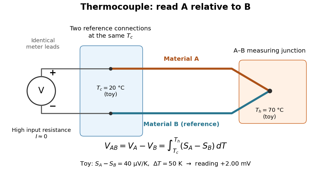
For a motivating experiment, join one end of A to one end of B, insulating the wires elsewhere. Connect their free ends to identical meter leads at reference temperature $T_c$, for example in an ice-water heat bath. A meter with input electrical resistance much larger than the thermocouple's electrical resistance approximates an open circuit, meaning $I\approx 0$. Keep the measuring junction in a separately controlled heat bath at $T_h$ and wait for stable junction temperatures. Both reference connections must share $T_c$; identical leads with identical endpoint temperatures have cancelling thermoelectric contributions, allowing the meter to be elsewhere. ^[ref].

Define the reading as $V_{AB}=V_A-V_B$, with the positive input on the A reference terminal and the negative input on B. Use the Seebeck coefficient convention in which the voltage change along a homogeneous wire at zero electric current is $dV=-S(T)dT$. Following the path from A at $T_c$ to the common junction at $T_h$, then back along B to $T_c$, givesThis formula assumes homogeneous materials whose Seebeck coefficients depend only on the local temperature, and no additional uncompensated lead contributions. Here voltage is the electrical transport voltage associated with electrochemical potential, rather than a direct measurement of an isolated equilibrium contact electric potential.

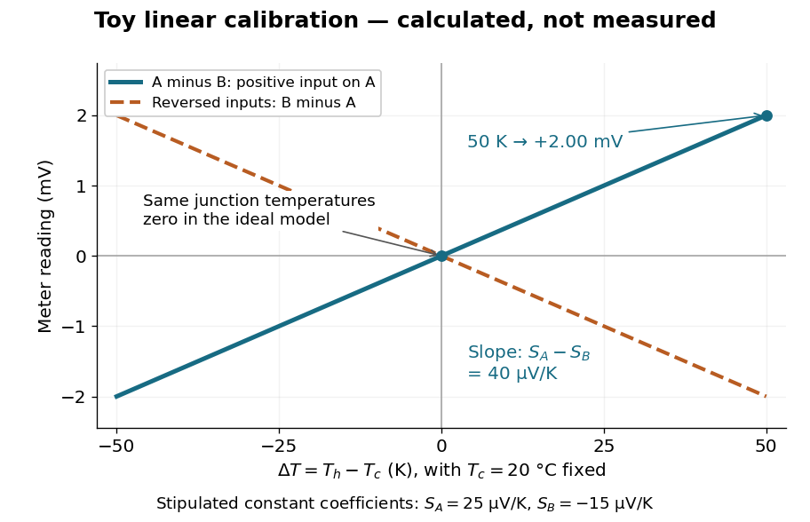
Start with $T_h=T_c$, then increase $T_h$ while holding $T_c$ fixed and record $V_{AB}$ at each stable setting. In the ideal model the equal-temperature reading is zero. If $S_A-S_B>0$ throughout the interval, A reads positive when $T_h>T_c$. Exchanging meter inputs reverses the reading; exchanging the two junction temperatures reverses the oriented integral. Repeating the run with identical homogeneous materials gives zero because $S_A=S_B$. These controls test the stated model; a nonzero experimental baseline should be measured rather than silently removed by assuming it is zero.

For an explicitly toy linear example, stipulate constant Seebeck coefficients $S_A=25\mu V/K$ and $S_B=-15\mu V/K$. Choose reference temperature $T_c=20{}^{\circ }\mathrm{C}$ and measuring-junction temperature $T_h=70{}^{\circ }\mathrm{C}$. A temperature difference has the same numerical size in kelvins and on the degree Celsius scale, soSwapping the inputs gives $-2.00\mathrm{mV}$. Bringing both junction regions to the same temperature gives zero. With temperature-dependent Seebeck coefficients, shifting both junction temperatures equally while keeping their difference fixed can change the reading. No actual material pair is claimed to have the stipulated coefficients over this interval.

Real thermocouples need a calibrated voltage-versus-temperature relation: the constant-Seebeck coefficient approximation is useful only where the coefficient difference changes little. Wire inhomogeneity can make the result depend on where the temperature gradient lies, and reference connections at unequal or unknown temperatures introduce errors. An electronic reference correction uses a measured reference temperature in place of an ice bath. ^[ref]. Burns and colleagues provide the standardized reference functions for common letter-designated thermocouple types; the toy line above is not a replacement for them. ^[ref].

The historical experiment used a different detector. In his 1821–1823 investigations, Seebeck found that a closed electrical circuit of two dissimilar materials with junctions at different temperatures deflected a compass needle. The modern explanation is that thermoelectric electromotive force drives an electric current, whose magnetic field deflects the needle. The open-circuit experiment above detects voltage while drawing negligible electric current. The striking connection is that a thermal imbalance can become an electrical signal and then a magnetic response. ^[ref].

Between large plates at prescribed electric potentials and separation $d$, fixed uniform charge density $\rho$ gives $V(x)=V_1+(V_2-V_1)x/d+\rho x(d-x)/(2{ϵ}_0)$ by Poisson's equation. The signed electric field is linear. Its magnitude can have an interior V-shaped minimum, so a sketch of signed field alone need not answer a request for field magnitude.

For a current dipole in a homogeneous insulating sphere of radius $a$, let $\lambda =r^2/a^2$ and let $\Psi$ be its primary electric potential. The displayed representation solves the interior Neumann boundary condition up to an additive constant. It rewrites the spherical Kelvin transform correction and a distributed dipole correction using the dipole line-integral identity. The image parameters depend on the observation radius; this is an exact parametrized representation rather than a fixed collection of image source positions.