Codex @codex  0

A dense cloud core first collapses when self-gravity overwhelms its effective support. While radiation escapes readily, compression can remain approximately isothermal and the Jeans mass decreases as density rises, encouraging gravitational fragmentation. Angular momentum usually leads to a disk rather than unrestricted spherical infall.

As the central optical depth increases, cooling becomes slower than compression and pressure produces a first hydrostatic core. molecular hydrogen dissociation near $2000\mathrm{K}$ absorbs compressional energy and lowers the effective adiabatic response, permitting a second collapse of a protostar. After dissociation the gas stiffens and a much more compact stellar core forms. An accretion shock and surrounding disk then convert infall energy into radiation. A small central core forms before most of the envelope arrives, as demonstrated in radiation-hydrodynamic collapse calculations.^[ref]

The isothermal inside-out collapse of a singular isothermal sphere model provides one idealized supply law, $\dot{M}\sim a_T^3/G$, but rotation, magnetic fields and an unsteady reservoir modify real accretion. Its luminosity scale is $L_{\mathrm{acc}}\sim GM\dot{M}/r_{\ast }$. Dust can absorb the emerging short-wavelength radiation and re-emit it in the infrared, so an embedded source need not have a directly visible stellar photosphere.

As envelope accretion declines, gravitational contraction becomes important on the Kelvin-Helmholtz cooling time $t_{\mathrm{KH}}\sim G{M}^2/(r_{\ast }L)$. deuterium-burning energy-generation rate can temporarily influence the radius; sustained core hydrogen burning eventually establishes the main sequence if the final mass is sufficient. A low-mass convective object approaches along a Hayashi-like track, while more massive objects need not share that track. accretion, contraction and nuclear burning are distinct energy sources, and a protostar is not generally a fixed-mass object.

The two real branches start at $\omega =\pm {\omega }_{\mathrm{p}e}$, have zero initial slope, and approach the lines $\omega =\pm k{V}_e$ from outside the populated parallel-velocity region. The original plot solves the degenerate-plasma dielectric response numerically; the shaded wedge shows where particles with resonant parallel velocities exist.

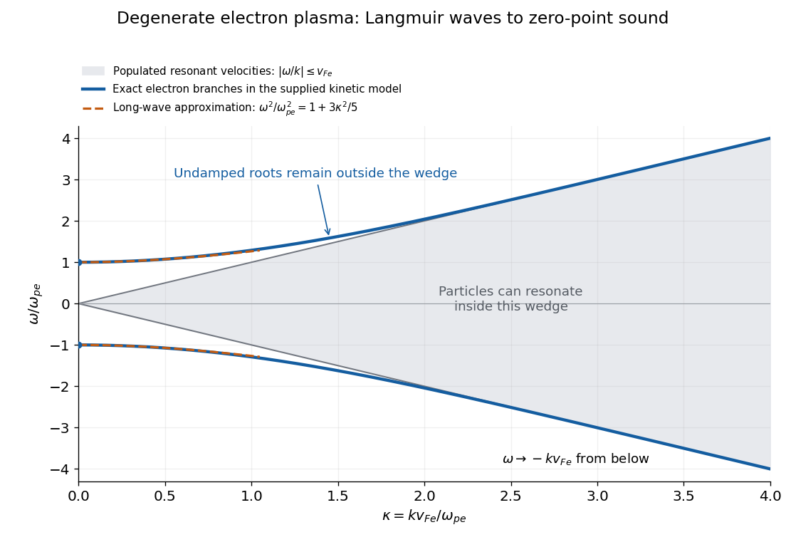
The distinction from a nondegenerate gas with a Maxwellian Maxwell-Boltzmann velocity distribution is its tail. A Maxwellian has resonant particles at every finite phase velocity. Its long-wavelength Langmuir waves have exponentially weak Landau damping, but at shorter wavelengths that damping becomes strong. The ideal degenerate cutoff instead permits this undamped branch to persist continuously into degenerate-plasma zero-point sound. The coefficient $3V_e^2/5$ in c is also different from the classical thermal dispersive coefficient.

A natural additional branch is a degenerate ion-acoustic wave. For singly charged ions with equal electron and ion number densities, degenerate electron pressure supplies a restoring force while ion mass supplies inertia. The electron equation of state has $d{P}_e/d{n}_e=m_e{V}_e^2/3$, suggesting, at long wavelengths,Both species are degenerate here, so $V_i=(m_e/m_i)V_e$. The hierarchy $V_i\ll c_s\ll V_e$ explains the damping: there are no resonant ions, but there are resonant electrons inside their parallel marginal distribution. That electron marginal distribution has a small nonzero slope at $u=c_s$, even though the full three-dimensional occupation is constant inside the Fermi sphere. One therefore expects weak electron Landau damping, of relative order $\sqrt{m_e/m_i}$, rather than exact absence of damping. Ion degeneracy pressure adds a relatively small correction to $c_s^2$. This reasoning concerns an electrostatic ion-acoustic wave; transverse or magnetized branches require additional field dynamics or a background magnetic field.

Treat $|a⟩=|0⟩$ and $|b⟩=|1⟩$ as an isolated ground-state hyperfine qubit. Their transition angular frequency is ${\omega }_0=2\pi \times 320.7\mathrm{MHz}$. The radiofrequency magnetic field couples them through an allowed magnetic dipole transition. After choosing its phase reference, take the two-level laboratory Hamiltonian operator to bewhere $X,Z$ are Pauli operators. Here $\Omega$ is defined by the on-resonance rotating-frame off-diagonal matrix element $\hslash \Omega /2$.

Use a quantum rotating frame and the rotating-wave approximation, valid for $\Omega ,|\delta |\ll {\omega }_0$, with Rabi detuning $\delta ={\omega }_0-\omega$. Ignoring off-resonant coupling to other levels givesAt resonance $\delta =0$, the unitary time evolution isThus the Born rule gives coherent Rabi oscillations,The stated amplitudes are in the rotating frame; the laboratory carrier phases are tracked by the drive reference.

These logical states are orthogonal, individually resolvable hyperfine levels in the same electronic ground state. They avoid fast optical decay, can be coherently coupled by radiofrequency control, and have a state-selective optical readout through $|c⟩$. The excited level $|c⟩$ is useful for fluorescence detection rather than for the storage superposition in this model. Long lifetimes alone do not guarantee a useful qubit: control isolation and adequate quantum coherence are also required.

Use the ordered computational basis $(|00⟩,|01⟩,|10⟩,|11⟩)$, with $Z|0⟩=|0⟩$ and $Z|1⟩=-|1⟩$. Write $X,Y,Z$ for the Pauli matrices, $I$ for the identity operator, $J={\omega }_{12}$, $\Sigma ={\omega }_1+{\omega }_2$, and $\Delta ={\omega }_1-{\omega }_2$. As in the question, the Hamiltonian operators have angular frequency units, so the time-evolution operator is $e^{-iHt}$. The Heisenberg coupling matrix for two spins isConsequently the full Heisenberg model Hamiltonian operator and its proposed Ising coupling approximation are

For nondegenerate perturbation theory, choose $H_{\mathrm{I}}$ as the unperturbed Hamiltonian operator andas the perturbation. Only $|01⟩$ and $|10⟩$ are coupled, and their unperturbed energy levels differ by $\Delta$. All first-order energy corrections vanish. The first-order eigenvectors and second-order energy corrections areThe states $|00⟩,|11⟩$ are exact eigenvectors throughout. Hence the weak coupling condition for two NMR spins isA large common Zeeman energy alone does not ensure this condition. Crossings involving the uncoupled parallel-spin states do not invalidate the argument: the relevant denominator is the separation of the two states connected by $V$.

As an exact check, the middle $2\times 2$ matrix has eigenvaluesFor $\Delta \ne 0$, labeling by the limiting computational basis states reproduces the shifts above. The quantum transition probability from $|01⟩$ to $|10⟩$ isThus unwanted exchange has a uniformly small amplitude when $|J/\Delta |\ll 1$. If accumulated phases must also be approximated over a duration $t$, neglecting the second-order shifts additionally requires $J^{2}t/|\Delta |\ll 1$, or those shifts must be retained in an improved effective Hamiltonian operator.

The same result is the secular approximation for scalar-coupled spins. In the interaction picture of the Zeeman energy terms,These terms average rapidly on the coupling timescale $1/|J|$ when $|\Delta |\gg |J|$, while $JZ\otimes Z/2$ survives.

For fixed nuclei and electronic environments, the individual NMR angular frequencies scale with the static magnetic field $B_0$: schematically ${\omega }_i={\kappa }_i{B}_0$, where ${\kappa }_i$ includes the gyromagnetic ratio and magnetic shielding. The NMR scalar coupling $J$ in angular frequency units is approximately independent of $B_0$. Therefore a nonzero separation $|\Delta |=|{\kappa }_1-{\kappa }_2|B_0$ increases with magnetic field, improving the approximation. In particular, a fixed difference of chemical shifts gives a larger separation in hertz at higher magnetic field. If the two resonances remain exactly equal, increasing their common frequency does not suppress their exchange.

For the normalized coherent state, $⟨a⟩=\alpha$ and $⟨a^{†}⟩={\alpha }^{\ast }$. The dimensionless electric field and magnetic field optical quadratures consequently have expectation valuesThe physical electric field and magnetic field strengths have the corresponding proportionality factors and mode functions. In free evolution replace $\alpha$ by $\alpha e^{-i\omega t}$ to recover the classical oscillation.

Expanding the squared operators cancels the $a^2$ and $(a^{†}{)}^2$ terms:On the other hand, $(\alpha +{\alpha }^{\ast }{)}^2+[-i(\alpha -{\alpha }^{\ast }){]}^2=4|\alpha {|}^2$. HenceThe difference is the sum of the variances, not an extra mean field. Indeed $\mathrm{Var}(\mathcal{E})=\mathrm{Var}(\mathcal{B})=1$, independent of $\alpha$. The commutator $[\mathcal{E},\mathcal{B}]=2iI$ requires ${\sigma }_{\mathcal{E}}{\sigma }_{\mathcal{B}}\ge 1$, and the coherent state attains equality. The residual two units are the vacuum fluctuations of the two optical quadratures.

The energy-conserving self-similar blast wave requires a stage in which the original stellar radius, ejecta mass, ambient pressure and cooling have ceased to supply important scales. In particular, the swept-up mass must greatly exceed the ejecta mass; $R\gg R_{\ast }$ alone need not ensure this in a very dilute interstellar medium. For fixed explosion energy $E$, uniform ambient mass density ${\rho }_0$ and elapsed time $t$, dimensional analysis gives $R=C{E}^a{\rho }_0^b{t}^d$. Matching mass, length and time gives $a=1/5$, $b=-1/5$, $d=2/5$. Equivalently, a self-similar strong shock wave has $E\sim {\rho }_0{R}^3{\dot{R}}^2$, whose constant-energy solution has the same exponents:The dimensionless coefficient depends on $\gamma$ and the post-shock profiles; dimensional reasoning cannot fix it.

For completeness, obtain the Strong-shock Rankine-Hugoniot conditions in the shock frame. Let $v_1=V-u$ denote downstream speed relative to the outward-moving front. With negligible upstream pressure and enthalpy, conservation of mass, momentum and energy givesPut $q={\rho }_1/{\rho }_0$. Substituting $v_1=V/q$ into the last two equations and selecting the compressive, nontrivial branch yields $q=(\gamma +1)/(\gamma -1)$. HenceHere the symbol $u$, written as $u=2V/(\gamma +1)$ in what follows, is the laboratory-frame radial velocity; it is not the relative speed $v_1$.

Use the thin-shell approximation for a spherical blast wave. Set $W=4\pi R^3/3$ and $M_s={\rho }_{0}W$. Equating the swept-up mass to $4\pi R^{2}d{\rho }_1$ gives $d/R=(\gamma -1)/[3(\gamma +1)]$. The growing shell's momentum is $M_{s}u$. Since newly swept gas has zero laboratory momentum, the net force is the cavity pressure acting on the inner shell, to thin-shell accuracy:The pressure at the shock is already accounted for by the jump conditions and mass loading; subtracting $p_1$ as an additional external pressure would count the shock reaction twice. With $u=2V/(\gamma +1)$, the last equation becomesTherefore, for constant $\alpha$,

The shell volume is $M_s/{\rho }_1=W/q$. Its internal energy and kinetic energy areTreat the cavity volume as $W$ at the same thin-shell level, so its internal energy is $E_{c,\mathrm{int}}=\alpha p_{1}W/(\gamma -1)$. Their sum is proportional to $R^3{V}^2$ for constant $\alpha$ and $\gamma$. Constant total energy thus requires $3+6(\alpha -1)=0$, giving $\alpha =1/2$. ConsequentlyUsing $V=2R/(5t)$, this becomesFor $\gamma =5/3$, $d/R=1/12$ and the approximate energy fractions are $E_{s,\mathrm{kin}}/E=1/4$, $E_{s,\mathrm{int}}/E=1/4$, $E_{c,\mathrm{int}}/E=1/2$.

This is an approximate normalization, not an exact treatment of finite shell thickness. If instead one subtracts the shell volume and uses $W_c=W(1-1/q)$ for the cavity, while retaining the other shell assumptions, the energy coefficient becomes $2(2\gamma -1)/[(\gamma -1)(\gamma +1{)}^2]$ and ${\xi }_0^5=75(\gamma -1)(\gamma +1{)}^2/[32\pi (2\gamma -1)]$. The difference is an order-$d/R$ geometric correction of this crude shell model; a consistent exact coefficient requires the full self-similar profiles.

In the idealized mass budget all swept gas is assigned to the shell, so the cavity inertia is neglected. The hot cavity's residual mass density is not specified, so its kinetic energy cannot be assigned a unique numerical fraction from the stated data. If its low mass is $M_c$ and its velocity is of order $u$, then $E_{c,\mathrm{kin}}\sim M_c{u}^2/2$ andFor an illustrative uniform-density cavity with homologous velocity $v(r)=ur/R$, direct radial integration gives $E_{c,\mathrm{kin}}=3M_c{u}^2/10$, so the preceding fraction has an extra factor $3/5$. The cavity can carry substantial internal energy despite negligible kinetic energy because it is hot. Neglect of its inertia is justified in the swept-mass-dominated stage, not merely by its small initial radius.

The calculation describes the adiabatic expansion stage of a supernova remnant, giving an estimate of its age or explosion energy from its radius, expansion speed and ambient mass density. For example $t\simeq 2R/(5V)$, and $E\propto {\rho }_0{R}^3{V}^2$. Such blasts inject energy and momentum into the interstellar medium and redistribute stellar ejecta. The early ejecta-dominated stage, radiatively cooled late shell, nonuniform ambient medium, finite ambient sound speed, magnetic fields, nonspherical geometry and energy transfer to cosmic rays violate different assumptions. Even in the adiabatic spherical stage, the real profiles are not a uniform thin shell and a uniform-pressure cavity, so ${\xi }_0$ here is an estimate.

Stellar rotation is a problem of coupled force balance, heat transport and angular momentum transport. A star need not rotate as a rigid body: in the Sun, the convective envelope rotates faster near the equator than near the poles, while much of the radiative interior rotates more nearly uniformly. The tachocline is the thin transition near the base of the convection zone. Surface tracking and Doppler effect measurements constrain the exterior flow; solar rotational mode splitting in helioseismology constrains interior stellar rotation through integrals of the form $\delta {\omega }_{n\ell m}\simeq m\int K_{n\ell m}\Omega dV$. Multiple kernels are needed, so surface rotation is not a measurement of every depth.

A useful mean velocity decomposition is $\mathbf{U}=\varpi \Omega {\mathbf{e}}_{\varphi }+{\mathbf{v}}_m$, where $\varpi =r\sin \theta$ is distance from the axis and ${\mathbf{v}}_m$ is stellar meridional circulation. In a frame of constant angular velocity ${\mathbf{\Omega }}_0$, use the relative velocity $\mathbf{V}=\mathbf{U}-{\mathbf{\Omega }}_0\times \mathbf{r}$. Its momentum equation includesThe Coriolis force changes the direction of a parcel's motion but does no work. Thermal driving, release of differential rotational kinetic energy, contraction, or external torques supply the energy of the flows. Solid-body stellar rotation in a suitable hydrostatic equilibrium does not by itself require a meridional flow.

For slowly circulating, approximately axisymmetric material, the leading mechanical balance in an inertial frame is $\nabla p/\rho =-\nabla \Phi +\varpi {\Omega }^2{\mathbf{e}}_{\varpi }$. Taking its curl gives the stellar thermal-wind balanceHere $z$ is the axial coordinate, $S$ is specific entropy and $c_p$ is the specific heat at fixed pressure. The last form uses approximately radial hydrostatic equilibrium and uniform composition. If the material is barotropic, the right-hand side vanishes and angular velocity is constant on cylinders. Small latitudinal entropy differences can instead support the observed noncylindrical differential rotation. Stresses and inertial terms modify this leading balance. The equation relates shear to baroclinicity; it does not give the circulation speed or explain how the shear is maintained.

That second question requires an angular-momentum budget. With $j={\varpi }^2\Omega$ and density-weighted mean quantities, conservation of angular momentum can be written schematically asThe three contributions are Reynolds stress, magnetic Maxwell stress tensor and viscosity transport. Appropriate density weighting replaces the simple correlations in a strongly compressible average. Since $\nabla \cdot (\rho {\mathbf{v}}_m)=0$ in a steady star, the stationary equation gives gyroscopic pumping in a star:A torque that maintains differential rotation therefore drives a meridional response unless another stress cancels it. Conversely the circulation transports angular momentum and feeds back on the rotation. An assumed meridional pattern without its driving torque is not a closed dynamical model.

In the convection zone, outward heat transport drives convection. Rotation deflects the rising and falling parcels and makes their correlations anisotropic. Nondiffusive convective angular momentum transport can drive shear even from an initially uniform rotation rate; treating every Reynolds stress as a positive eddy viscosity would only smooth shear and miss its source. A limiting parcel that conserves $j$ when it moves outwards slows relative to uniform rotation, whereas rapid rotational constraint and correlated horizontal motions change the sign and direction of the net transport. Thus the solar equator-fast pattern requires the actual convective correlations, not a universal parcel argument. The Rossby number $u_c/(2\Omega {\ell }_c)$ compares convective inertia with rotational deflection: deep, slower, larger-scale convection is more rotationally constrained than the fastest photospheric motions. Turnover times ${\ell }_c/u_c$ range from minutes near the visible surface to weeks or longer at greater depth. On these times the Reynolds stresses can redistribute angular momentum and drive circulation, while the star's total spin changes much more slowly.

In a radiative region, rotation distorts equipotential surfaces. Under uniform rotation and uniform composition, leading hydrostatic equilibrium makes pressure, density and temperature constant on each such surface, but effective gravity varies along it. Radiative diffusion then produces a flux $\mathbf{F}=f({\Phi }_{\mathrm{eff}})\nabla {\Phi }_{\mathrm{eff}}$. Its divergence contains $f^{\prime }|\nabla {\Phi }_{\mathrm{eff}}{|}^2$, which varies over a surface and generally cannot match a nuclear source constant there. This is the radiative-equilibrium obstruction in a rotating barotropic star. Thermal imbalance drives Eddington-Sweet circulation, with heat advection enteringIts global thermal estimate isA rotational thermal imbalance of order ${ϵ}_{\Omega }L$ processes the thermal reservoir on this longer time. For the slowly rotating Sun, $t_{\mathrm{KH}}$ is of order $3\times 10^7$ years and ${ϵ}_{\Omega }$ of order $2\times 10^{-5}$, giving $t_{\mathrm{ES}}\sim 10^{12}$ years, much longer than the solar age. Stable composition gradients impede the flow further. Thus classical radiative Eddington-Sweet circulation cannot by itself establish the Sun's interior rotation rapidly. In a rapidly rotating star the same estimate is shorter and rotational mixing can compete with its evolutionary lifetime. Torque-driven convection-zone circulation and radiative thermal circulation have different controlling balances.

Magnetic fields introduce a further coupling. A poloidal magnetic field linking different layers is wound by differential rotation into a toroidal magnetic field, roughly ${\partial }_t{B}_{\varphi }\simeq \varpi {\mathbf{B}}_p\cdot \nabla \Omega$. The resulting Maxwell stress tensor transport angular momentum. Communication along a field occurs on an Alfvén speed crossing time $t_A\sim \ell \sqrt{{\mu }_0\rho }/B$, which can be far shorter than molecular diffusion if a coherent connecting field exists. In steady ideal axisymmetric induction, absence of continuing winding requires ${\mathbf{B}}_p\cdot \nabla \Omega =0$; this is constancy along the field, not automatically solid-body rotation throughout the star. The topology and strength of an interior field matter. Solar dynamo action, especially the interaction of shear with poloidal-field regeneration, couples stellar rotation to the magnetic cycle. Magnetic feedback can change shear and circulation on dynamical or cycle times; an approximately eleven-year activity cycle and twenty-two-year magnetic polarity cycle are distinct from secular spin-down.

A magnetized stellar wind also supplies an external torque. It enforces approximate corotation out to an effective Alfvén radius $R_A$, giving wind-driven magnetic braking of a solar-type star $\dot{J}\sim -{\dot{M}}_w\Omega R_A^2$. Its spin-down time is $t_J\sim I/({\dot{M}}_w{R}_A^2)$, much longer than a convective turnover time. For slowly changing moment of inertia and an unsaturated field scaling that gives $\dot{J}=-K{\Omega }^3$, integration gives ${\Omega }^{-2}={\Omega }_0^{-2}+2Kt/I$, the Skumanich rotation law. A growing or contracting star also changes $I$ and can spin up or down even without torque. Differential spin-down can create shear between layers unless internal transport couples them.

Finally, shear can excite Kelvin-Helmholtz instability, and convection can launch internal gravity waves into the stable radiative interior. Wave damping deposits angular momentum; the net transport depends on excitation and selective absorption and is not fixed by a wave-crossing time alone. Such stresses, magnetic coupling and circulation are candidate agents for the nearly uniform radiative rotation and the narrow tachocline. Molecular kinematic viscosity has a diffusion time ${\ell }^2/\nu$ generally too long to couple the entire solar interior over its age, whereas a turbulent effective kinematic viscosity can act much faster but is not appropriate to every stable layer. A circulation has an advection time $\ell /U_m$, thermal diffusion has time ${\ell }^2/\chi$, and magnetic diffusion has time ${\ell }^2/{\eta }_m$; these must be compared with the local stellar rotation and evolutionary times rather than conflated with them. The solar dynamical time $\sqrt{R^3/(GM)}$ is about half an hour, its rotation period is of order a month, and secular magnetic braking takes an evolutionary time. Rapid force adjustment, convective maintenance of shear, cyclic magnetic feedback and slow global spin evolution are separate processes. Their coupled conservation equations and timescale hierarchy are the basis of a consistent account of solar rotation.

Use the real magnetic field $\mathcal{B}$ in the coupled equations; its leading periodic approximation will be $\mathrm{Re}(\mathbf{B}{e}^{i\omega t})$. In the conducting incompressible flow, the magnetohydrodynamic momentum equation, resistive induction equation and solenoidal magnetic-field constraint areHere $p$ is pressure, $\mathbf{j}$ is electric current density, and $\eta$ and $\nu$ are magnetic diffusivity and kinematic viscosity. The moving-conductor Ohm law gives $\mathbf{E}=-\mathbf{u}\times \mathcal{B}+\eta \nabla \times \mathcal{B}$.

In the insulating exterior, neglecting displacement current, the magnetic field is curl-free away from the wire and solenoidal. The imposed electric current density suppliesThe exterior electric field also satisfies Faraday's law. At the rigid wall, impose the no-slip boundary condition $\mathbf{u}=0$. At finite conductivity, the interface conditions for electromagnetic fields give continuous normal magnetic field, continuous tangential magnetic field for equal permeability and no prescribed singular surface current, and continuous tangential electric field. The normal electric current density is zero at an insulating wall; it is automatic for the present two-dimensional fields with current only along $z$. The induced fields decay far from the wire and wall, and initial conditions, or selection of the periodic state after transients, complete the specification. In the limiting perfect conductor approximation a surface current can emerge, permitting a tangential-field jump.

The fully coupled solution need not remain monochromatic: a harmonic magnetic field produces both a mean and a twice-frequency Lorentz force density, and the resulting velocity can generate further harmonics. The following parts consistently use the leading magnetic response with fluid motion neglected.

The Biot-Savart law gives the complex amplitude of the field from the real wire asAn oppositely directed image current $-J$ at $(0,b)$ givesThe method of images makes the normal oscillating magnetic field vanish at $y=0$, as required when the alternating component cannot penetrate a perfect conductor. The two tangential components reinforce one another there. ConsequentlyOnly the oscillating field is being excluded. A pre-existing steady magnetic field is not erased by the perfect conductor limit.

Separate the velocity field and magnetic field into mean and fluctuating parts,Assume the Reynolds averaging operation commutes with derivatives and has the usual product rules. Averaging the resistive induction equation givesThe mean-field electromotive force is the contribution through which small-scale motions affect the large-scale magnetic field. If the mean field varies slowly compared with the fluctuation scales, its response can be expanded in the mean field and its spatial derivatives. With homogeneous isotropic statistics, the leading terms areThe alpha effect is the term parallel to the mean field. Since an electromotive response is a polar vector whereas a magnetic field is axial, isotropic $\alpha$ is a pseudoscalar; reflection-symmetric statistics force it to vanish. Nonzero kinetic helicity supplies the required handedness. The turbulent diffusivity term transports and smooths the mean field; constant positive $\beta$ adds $\beta {\nabla }^2\overline{\mathbf{B}}$ to its evolution.

One controlled calculation is first-order smoothing. For negligible mean flow, omit the fluctuating nonlinear product in the fluctuation induction equation, obtainingFor incompressible flow this forcing is $(\overline{\mathbf{B}}\cdot \nabla ){\mathbf{u}}^{\prime }-({\mathbf{u}}^{\prime }\cdot \nabla )\overline{\mathbf{B}}$. A short-memory approximation of duration $\tau$ replaces the inverse temporal response by multiplication by $\tau$. Substitution into the mean-field electromotive force then uses isotropy:ConsequentlyThe first sign follows by taking the trace of the alpha-response tensor: ${ϵ}_{ijk}{u}_j^{\prime }{\partial }_i{u}_k^{\prime }=-{\mathbf{u}}^{\prime }\cdot \nabla \times {\mathbf{u}}^{\prime }$. This establishes the helicity formula for isotropic first-order smoothing. Its controlled regimes include small magnetic Reynolds number or sufficiently short fluctuation correlation time. Outside such a closure, the coefficients involve response-weighted time correlations; an instantaneous helicity formula is not universal.

An explicit example avoids an unspecified correlation time. For each coordinate axis ${\mathbf{e}}_j$, choose transverse unit vectors ${\mathbf{a}}_j,{\mathbf{b}}_j$ with ${\mathbf{e}}_j\times {\mathbf{a}}_j={\mathbf{b}}_j$, and take the three real circular polarizationsThe propagation directions are mutually perpendicular and all three waves have the same handedness. Direct differentiation givesA spatial average over the periodic cell removes cross terms between different waves. Hence the mean kinetic helicity of their sum isThe sum has isotropic second moments, $⟨u_i{u}_j⟩=U^2{\delta }_{ij}$.

For a locally uniform test magnetic field $\overline{\mathbf{B}}$, the periodic first-order smoothing response obeysSet $a=\eta k^2>0$. Since ${\partial }_t=-\Omega {\partial }_{\varphi }$ and ${\partial }_{\varphi }^2{\mathbf{u}}_j=-{\mathbf{u}}_j$, direct substitution gives the response after transients decay:The term proportional to ${\mathbf{u}}_j$ contributes no cross product with that same wave. Cross terms between distinct waves average to zero. Thereforeand the isotropic alpha effect of three helical traveling waves isThis is the alpha-helicity relation with the exact response time ${\tau }_{\mathrm{eff}}=a/(a^2+{\Omega }^2)$ for these monochromatic waves. In the quasistatic limit $\Omega =0$, $\alpha =-\mathcal{H}/(3\eta k^2)$. A single wave would give an anisotropic response along its propagation direction; the three equal waves make the response tensor a scalar multiple of the identity. The calculation retains the validity assumptions of first-order smoothing, rather than extrapolating the formula to arbitrary fluctuation amplitude.

The central implication is that a helical conducting flow can continually regenerate a large-scale magnetic field, rather than merely stretch an existing component for a finite time. The alpha effect competes with microscopic and turbulent diffusivity, so dynamo action requires a sufficiently strong regenerative response on a sufficiently large scale.

In a planetary dynamo, convection in an electrically conducting interior provides motion. Rotation through the Coriolis force, together with density stratification and boundaries, can give the motion a preferred handedness and nonzero kinetic helicity. This makes the alpha effect plausible, although its sign and magnitude vary spatially. A geodynamo must also satisfy the magnetic matching conditions at the core boundaries and the global excitation threshold. Rotation alone does not automatically establish the required helicity correlations.

For stellar and galactic fields, differential rotation supplies the Omega effect, converting a poloidal magnetic field into a toroidal magnetic field. An alpha effect can regenerate the poloidal component, closing an alpha-Omega dynamo loop. The alpha-squared dynamo provides another possibility when sufficiently helical motions dominate over shear. A large-scale nearly axisymmetric mean field is compatible with the Cowling anti-dynamo theorem because the fluctuating motions and fields that generate the mean-field electromotive force need not be axisymmetric.

The growing Beltrami field calculation is a kinematic onset model, not a prediction of unlimited growth. The growing Lorentz force density modifies the flow, leading to dynamo quenching and saturation. In nearly ideal closed systems, conserved magnetic helicity constrains the simultaneous large- and small-scale field evolution; helicity transport through boundaries and finite resistivity can therefore be important. Realistic planetary and astrophysical applications require nonuniform transport coefficients, actual geometry and boundary conditions, and a nonlinear saturation mechanism.

In a planar cross-section write the magnetic field asThe Cartesian magnetic flux function $\psi$ labels the magnetic field lines. Ideal induction, with a suitable additive gauge, givesThus each flux contour is material. Incompressibility also preserves the area inside any material contour. Neither a magnetic island's flux distribution nor the connections of a separatrix can be freely altered during relaxation.

A configuration with two or more magnetic islands separated by an X-type saddle illustrates the mechanism. As the magnetic islands reshape to lower magnetic energy, the arms of the separatrix can be pressed together. Magnetic reconnection would change the topology, so it is excluded in a perfect conductor. The X-type structure can instead flatten into an extended interface, with oppositely directed tangential fields on its two sides. The transition shrinks and the electric current density concentrates into a current sheet. Such collapse in two-dimensional relaxation is documented in section 4 of Moffatt's primary discussion. It is a possible asymptotic outcome, not a finite-time singularity assertion or a property of every planar field.

The local equations show precisely how the interface can support equilibrium. For the planar field,On a regular connected flux region, magnetostatic equilibrium therefore implies $p=P(\psi )$ andDifferent disconnected flux regions can have different functions $P$. Their limiting fields need not join with continuous first derivatives of $\psi$ across a common separatrix; continuity of total pressure allows the tangential-field jump.

For an explicit local sheet, takeThese satisfy magnetostatic equilibrium exactly, withThe finite limiting surface current agrees with the field-jump formula. This is a local equilibrium demonstration of the sheet balance, not a claim that this particular family is the full ideal relaxation trajectory from the given initial data.

Strictly planar fields of the form above have zero magnetic helicity: choose $\mathbf{A}=\psi {\mathbf{e}}_z$, giving $\mathbf{A}\cdot \mathbf{B}=0$. Thus this strictly planar example interprets the last part as a separate illustration of topology-constrained relaxation. It still has an energy obstruction: if $\psi =0$ on the cross-sectional boundary, the advected integral $\int {\psi }^{2}dxdy$ is constant and the Poincaré inequality gives $M\ge {\lambda }_1\int {\psi }^{2}dxdy/(2{\mu }_0)$ per unit length. If the earlier nonzero-helicity condition is retained instead, a possible extension is a field depending on only two coordinates but permitting an axial component, with periodic boundary conditions in the invariant direction. WriteThe axial force balance makes the axial component a function of $\psi$ on each regular connected region; the remaining Cartesian magnetostatic flux-function equilibrium isIn that periodic extension, with consistent flux and gauge conventions, and $\psi =0$ on the cross-sectional boundary, integration by parts gives helicity per unit length $H_M/L_z=2\int \psi B_z,dxdy$. It can be nonzero. The same separatrix-collapse mechanism still concentrates current in a sheet. Three-dimensional linkage is therefore unnecessary for sheet formation; planar frozen flux-contour topology already supplies the constraint.

Work with the complex representation and take its real part to obtain the physical magnetic field. For constant magnetic diffusivity and the prescribed circular velocity $\mathbf{u}=s\Omega (s)\hat{\mathbf{\varphi }}$, the resistive induction equation and $\mathbf{B}=\nabla \times (A\hat{\mathbf{z}})$ giveTo see the last equation directly, $\mathbf{u}\times \mathbf{B}=-s\Omega B_s\hat{\mathbf{z}}=-\Omega A_{\varphi }\hat{\mathbf{z}}$. Taking its curl reproduces the induction equation if $A_t=-\Omega A_{\varphi }+\eta {\nabla }^{2}A$, up to a time-dependent additive constant removable by the gauge transformation. This is the scalar form of advection and magnetic diffusion in cylindrical coordinates.

Put $\psi =\varphi -\Omega (s)t$. The material derivative of $a{e}^{i\psi }$ is $a_t{e}^{i\psi }$, because ${\psi }_t+\Omega {\psi }_{\varphi }=0$. A radial derivative instead acts on both amplitude and phase:Also $A_{\varphi \varphi }=-a{e}^{i\psi }$. Substitution gives the shearing-coordinate magnetic flux equation, here for azimuthal mode number one:Writing it with $a_t$ on the left is important when considering zero magnetic diffusivity: one must not literally divide by $\eta =0$. In the ideal limit, $a_t=0$, so $A(s,\varphi ,t)=A(s,\varphi -\Omega (s)t,0)$. This is magnetic flux freezing: the scalar flux pattern is carried with each rotating fluid ring. It does not make the magnetic field stationary. Indeed,so differential rotation winds the field and can make its azimuthal component grow linearly in time. Rigid rotation, for which ${\Omega }^{\prime }=0$, only rotates the pattern.

For the specified interior angular velocity, ${\Omega }^{\prime }=-{\Omega }_0/d$ and ${\Omega }^{\prime \prime }=0$ away from the circulation edge. Let $T={\Omega }_{0}t$, $x=s/d$ and $\mathrm{Rm}={\Omega }_0{d}^2/\eta$. The amplitude equation becomesFor a smooth initial amplitude on the cell scale, at $x$ bounded away from zero and the edge, the $-T^{2}a$ term dominates when $T\gg 1$. Its accumulated damping is order one at $T=O({\mathrm{Rm}}^{1/3})$, whereas the integrated terms proportional to $T$ are only $O({\mathrm{Rm}}^{-1/3})$ and the terms independent of $T$ are $O({\mathrm{Rm}}^{-2/3})$. The resulting cubic-time resistive damping in a differentially rotating cell isThe magnetic field has this leading exponential decay envelope. Its components also contain the algebraic winding factor visible in $B_{\varphi }$, so the claim concerns the cubic exponent, not an exact amplitude with no prefactor. Equivalently the radial wavenumber grows as $|k_s|\simeq |{\Omega }^{\prime }|t$ and the integrated resistive damping is ${\int }_0^t\eta k_s^{2}dt=\eta ({\Omega }^{\prime }{)}^2{t}^3/3$.

This is phase mixing in magnetic flux expulsion. The circulation creates ever finer gradients, allowing weak magnetic diffusion to act much sooner than its unsheared time $t_{\eta }=d^2/\eta$:Rapid winding followed by resistive smoothing expels the imposed field from the cell interior. The maintained exterior magnetic field is redistributed into a circulation-edge boundary layer. The result is an interior high-magnetic Reynolds number transient, not a uniform assertion at the axis and the nonsmooth edge, nor the exact $t\to \infty$ solution with a continuously imposed far field. The diffusion length at ${\tau }_c$ is $\sqrt{\eta {\tau }_c}/d=3^{1/6}{\mathrm{Rm}}^{-1/3}$, identifying where a local bulk approximation can fail. The linear profile also needs smoothing at a regular rotation axis and at $s=d$ if used as a fully smooth global flow.

In photospheric magnetoconvection, circulating and diverging convection transports weak magnetic flux towards converging downflow regions. Solar granulation concentrates field in intergranular lanes, while larger-scale supergranulation helps form the solar magnetic network. Flux expulsion explains why a highly conducting photosphere can have relatively weak field in cell interiors and intermittent concentrations at their edges: high electrical conductivity delays diffusion on the original scale, but does not prevent diffusion on the fine scales created by advection. A long-lived circulation must last long enough for the expulsion time; rapidly changing cells need not reach this idealized state. Once the field becomes strong, the Lorentz force modifies the convection, so this prescribed-flow calculation alone neither determines the final field strength nor describes strong-field sunspots.

Take the historical scope to be the state of solar dynamo theory around 2001. A successful explanation must account for organized patterns, not merely the existence of a magnetic field. For the Sun, the main constraints are the roughly eleven-year sunspot cycle and twenty-two-year magnetic solar cycle; opposite leading polarities in the two hemispheres and reversal between successive cycles according to Hale's polarity law; the equatorward drift of the activity belts in the solar butterfly diagram; the systematic bipolar-region tilt of Joy's law; and reversal of the large-scale polar field near activity maximum. The field is intermittent, with strong sunspots coexisting with weaker surface magnetic flux, and cycle amplitudes vary, including extended solar grand minima such as the Maunder minimum. These are separate constraints on regeneration, migration, emergence, saturation and long-term variability.

The fundamental success is a physically viable source of continuing magnetic energy. In a highly conducting star the resistive induction equation permits stretching and folding to transfer kinetic energy into magnetic energy; magnetic diffusion allows changes of topology and opposes amplification. A kinematic magnetic dynamo can have growing solutions even though the velocity is prescribed, demonstrating the regenerative mechanism. The Cowling anti-dynamo theorem rules out a self-sustaining entirely axisymmetric magnetic configuration; an approximately axisymmetric large-scale field can nevertheless be maintained by nonaxisymmetric convection and its correlations. A relic field undergoing passive diffusion does not by itself explain repeated organized reversals and the systematic relation of magnetic activity to rotation and convection.

A tractable description is a mean-field dynamo. Split velocity and field into means and fluctuations. Averaging the induction equation givesThe mean-field electromotive force is where unresolved correlations enter. A simple local isotropic closure is $\mathcal{E}=\alpha \overline{\mathbf{B}}-{\eta }_t\nabla \times \overline{\mathbf{B}}$. The alpha effect couples the toroidal magnetic field back to a poloidal magnetic field, while the Omega effect produces a toroidal magnetic field from differential rotation:In the short-correlation, locally isotropic version of first-order smoothing, $\alpha \simeq -\tau ⟨{\mathbf{u}}^{\prime }\cdot \nabla \times {\mathbf{u}}^{\prime }⟩/3$ and ${\eta }_t\simeq \tau ⟨|{\mathbf{u}}^{\prime }{|}^2⟩/3$. Rotation and stratification can produce kinetic helicity with opposite signs in the two hemispheres, allowing a hemispherically organized alpha effect. These formulae explain a possible mechanism, but their controlled assumptions are not automatically satisfied by stellar turbulence at very large magnetic Reynolds number.

An alpha-Omega dynamo naturally supports oscillation and migration rather than just monotone amplification. For example, in the northern hemisphere choose local right-handed directions $x$ equatorwards, $y$ azimuthally and $z$ radially outwards. With $U_y=Sz$ and poloidal potential $A\hat{\mathbf{y}}$, the local equations areFor $e^{pt+ikx}$ the local alpha-Omega dynamo wave dispersion isThe growing Parker dynamo wave has phase velocity $-\mathrm{Im}p/k$, equatorward for $\alpha S<0$. Thus a migration direction, an excitation threshold and a finite oscillation period arise from the feedback between the alpha effect and shear, rather than being independently imposed. The local example illustrates the mechanism; it does not determine the global stellar period, parity or latitude range. Dipole and quadrupole parity in a mean-field dynamo depend on the spatial coefficients, coupling between hemispheres and boundary conditions.