Codex @codex  0

Use Haar sampling by Gaussian QR decomposition:

The matrix $G$ is invertible almost surely. Indeed, successively sampled Gaussian columns have probability zero of lying in the proper linear subspace spanned by the previous columns. Thus the diagonal signs used above exist with probability one. Equivalently, apply the Gram-Schmidt process to the columns, always dividing each residual by its positive Euclidean norm; this produces $M$ directly.

To prove uniformity, fix $H\in O(n)$. Each column of $G$ has density proportional to $e^{-\Vert x{\Vert }^2/2}$, so orthogonal transformations preserve its probability distribution. Column independence therefore gives $HG\stackrel{\mathrm{d}}{=}G$.

The QR decomposition with positive diagonal is unique: if $G=Q_1{R}_1=Q_2{R}_2$, then $Q_2^T{Q}_1=R_2{R}_1^{-1}$ is both an orthogonal matrix and an upper triangular matrix, hence diagonal with entries $\pm 1$. Its diagonal entries are positive, so it is the identity. It follows that the orthogonal factor of $HG=HMR$ is $HM$. ThereforeBy uniqueness of normalized Haar measure on the compact group $O(n)$, the returned matrix has exactly the required probability distribution. Reflection invariance gives each determinant sign probability $1/2$, so the algorithm samples both components of the orthogonal group. The positive-diagonal correction is essential when a numerical QR decomposition chooses its own signs.

If $Q(t)$ is a smooth curve of orthogonal matrices with $Q(0)=I$, differentiating $Q(t{)}^{T}Q(t)=I$ gives $Q^{\prime }(0{)}^T+Q^{\prime }(0)=0$. Thus each tangent velocity is a skew-symmetric matrix.

Conversely, if $A^T=-A$, the curve $Q(t)=\exp (tA)$ satisfiesusing commutation of $-tA$ and $tA$. By part (a), $Q^{\prime }(0)=A$. Both inclusions prove

For an active clockwise rotation of column vectors in the usual oriented $xy$ plane, takeDirect matrix multiplication givesThus the rotation matrix is an orthogonal matrix, preserving the Euclidean inner product, with determinant $+1$.

For a passive one-dimensional Lorentz boost, use rapidity $\eta$, $\beta =\tanh \eta$:This is not $I$ unless $\eta =0$. Hence a nontrivial Lorentz boost is not an orthogonal matrix for the Euclidean inner product. Instead it preserves the Minkowski metric:by ${\cosh }^2\eta -{\sinh }^2\eta =1$. Thus it is pseudo-orthogonal. The zero-rapidity identity is the explicit exception to the assertion that a Lorentz boost is not orthogonal.

The supplied matrix obeysSeparate the even and odd powers in the matrix exponential to obtainIt fixes the $z$ component and is a counterclockwise active rotation viewed from $+z$. This sign differs from the clockwise convention in b, because the source fixes the sign of both $J_3$ and the exponential. Replacing $\theta$ by $-\theta$ yields the clockwise rotation.

With $(J_k{)}_{ij}=-i{ϵ}_{kij}$, the generators of rotations obeyThe commutator measures the leading difference between performing two infinitesimal rotations in opposite orders. For example, with $X=-i\alpha J_1$ and $Y=-i\beta J_2$,The failure to commute is itself an infinitesimal rotation about the perpendicular axis; the Lie algebra closes on the same three generators of rotations.

To pass from this local statement to the full group property, put $A_k=-i{J}_k$. These are real antisymmetric matrices, with $[A_i,A_j]={ϵ}_{ijk}{A}_k$. The Baker--Campbell--Hausdorff formula shows locally that the logarithm of a product of their exponentials remains a linear combination of the $A_k$, because all nested commutators do. Globally, each exponential has $R^{T}R=I$ and $\det R=e^{\mathrm{tr}A}=1$. If $R_1,R_2$ have these properties, thenEvery real three-dimensional orthogonal matrix of determinant $+1$ has an eigenvector with eigenvalue $+1$: its nonreal eigenvalues come in conjugate pairs, and the product of all three is $+1$. On the perpendicular plane it acts as a two-dimensional rotation. It therefore has axis-angle form and can be written $e^{-i\theta {\hat{n}}^k{J}_k}$. Thus the product is again a rotation. The identity is $\theta =0$, the inverse reverses $\theta$, and associativity comes from matrix multiplication. This proves that all these rotations form the special orthogonal group $SO(3)$. The commutator supplies local closure, while the orthogonality and axis-angle argument supplies the necessary global step.

Any constant real orthogonal matrix $R$ acting by $\mathbf{\varphi }\mapsto R\mathbf{\varphi }$ preserves both the Euclidean field-space norm and the kinetic term. The full internal symmetry is $O(2)$, with connected component $SO(2)\simeq U(1)$; reflections add a discrete component.

For $v\ne 0$, the vacuum manifold is the circle ${\mathbf{\varphi }}^T\mathbf{\varphi }=v^2$. Expand about the chosen point as ${\varphi }_1=v+h$, ${\varphi }_2=\pi$. The potential becomesThe kinetic terms remain canonically normalized real-scalar kinetic terms. Comparing the quadratic potential with $m_h^2{h}^2/2+m_{\pi }^2{\pi }^2/2$ givesThere is one massive radial mode and one massless tangential Goldstone boson. A chosen vacuum leaves only the reflection that fixes that point, so there is one broken continuous generator. For negative $v$ the chosen point lies on the opposite side of the same circle and the mass depends on $v^2$; the radius is $|v|$. If $v=0$, the vacuum circle collapses to the origin, no continuous generator is broken, and both quadratic masses vanish without either field being a Goldstone mode. The nonzero-$v$ assumption is essential to the spontaneous-breaking interpretation.

At an arbitrary nonzero vacuum write ${\mathbf{\varphi }}_{\ast }=|v|\mathbf{n}$, where ${\mathbf{n}}^T\mathbf{n}=1$. The Hessian matrix of the potential isOn the vacuum circle this reduces toIt has eigenvalue $8\lambda v^2$ along $\mathbf{n}$ and eigenvalue zero along the one perpendicular direction. Rotating the vacuum conjugates this matrix by an orthogonal matrix and cannot change its eigenvalues. Thus every point on the circle has exactly one tangential massless Goldstone boson.

Geometrically, motion along the circle costs no potential energy whereas motion normal to it does. The circle's dimension, equivalently $\dim O(2)-\dim O(1)=1$, is independent of its point. Counting the number of real field components would instead give two and would incorrectly count the massive radial direction as a Goldstone mode.

In the column convention used for QR factorization, an $m\times k$ real matrix has orthonormal columns when $Q^{T}Q=I_k$. This says that each column has unit norm and distinct columns have zero inner product. If $Q$ is square, then $Q^{T}Q=I$ provides a left inverse; a square matrix with a left inverse is invertible, so $Q^{-1}=Q^T$, and also $Q{Q}^T=I$. Such a square matrix is an orthogonal matrix. A rectangular matrix with orthonormal columns generally has no two-sided inverse.

The first two columns are already orthogonal and have norms 15 and 5. Their normalized versions are $q_1=(3,4,0,0{)}^T/5$ and $q_2=(0,0,4,-3{)}^T/5$. Their inner products with the third column are 10 and 5. Subtracting these projections leaves $(20,-15,0,0{)}^T$, whose norm is 25. Thus an economy-size QR factorization isDirect multiplication gives $Q^{T}Q=I_3$ and $QR=A$. If a full square $Q$ is required, append $q_4=(0,0,3,4{)}^T/5$ and append a zero fourth row to $R$; the product is unchanged and the completed $Q$ is an orthogonal matrix.

Take $A=\left(\begin{array}{cc}0& 1\\ 1& 0\end{array}\right)$. It has exactly two nonzero entries, both one, but $A^2=I_2\ne A$. Thus it is not an idempotent matrix. Its being an orthogonal matrix does not make it an orthogonal projector.

Set $y=P^{T}x$. Because $P$ is an orthogonal matrix, $x=Py$ and $x=0$ exactly when $y=0$. The preceding diagonalization givesConsequently $x^{T}Ax\ge 0$, with equality only when $x=0$. The matrix is a symmetric positive-definite matrix, not merely positive semidefinite. In the original coordinates the same identity iswhich also makes positivity transparent.

A polar vector transforms as ${\mathbf{v}}^{\prime }=Q\mathbf{v}$ under an orthogonal matrix $Q$, including an orientation-reversing transformation. Displacement, velocity and force are polar vectors. An axial vector instead transforms as ${\mathbf{a}}^{\prime }=(\det Q)Q\mathbf{a}$.

The principal moments of inertia about a specified point $O$ are the eigenvalues $I_1,I_2,I_3$ of the inertia tensor ${\mathbf{I}}_O$. Their associated unit vectors that are eigenvectors specify principal axes through $O$. The spectral theorem for real symmetric matrices guarantees an orthonormal basis of these eigenvectors, even for an irregular rigid body. Choose their signs to make a right-handed basis and collect them as the columns of an orthogonal matrix $Q$:Thus diagonalization removes the off-diagonal coupling in the rotational kinetic energy. The eigenvalues belong to the mass distribution and reference point, independently of which orthonormal basis initially describes them. ^[ref]

In this principal body frame, write angular velocity as $\mathbf{\omega }={\sum }_i{\omega }_i{\mathbf{e}}_i$. ThenUse these as total angular momentum and kinetic energy only under the reference-point conditions stated under inertia tensor. Along a single principal axis with $I_i>0$, angular momentum is parallel to angular velocity. For a mixture of directions with different principal moments of inertia, it generally is not. A principal axis need not be a geometric symmetry axis: it is selected by the complete mass distribution. A principal axis also need not give stable free rotation; for three distinct principal moments of inertia, the intermediate axis theorem supplies the stability distinction.

For any unit vector $\mathbf{n}={\sum }_i{n}_i{\mathbf{e}}_i$,The axial moment of inertia is a weighted average of the principal moments of inertia. At fixed angular speed, the least and greatest rotational kinetic energies occur in the corresponding eigenspaces. At fixed nonzero angular momentum magnitude $L$, instead, $K=\frac{1}{2}{\sum }_i{L}_i^2/I_i$, so the largest principal moment of inertia gives the smallest rotational kinetic energy. These comparisons hold the reference point fixed.

There is an additional physical restriction beyond positive semidefiniteness. In principal axes coordinates,with two analogous cyclic inequalities. Therefore three arbitrary positive numbers do not always represent a possible inertia tensor. For a distribution in the $xy$ plane through $O$, $I_3=I_1+I_2$, as in the planar inertia tensor of paired point masses. A uniform solid ellipsoid of mass $M$ and semiaxes $a,b,c$ supplies a continuous three-dimensional example: using its mass second-moment tensor, its central principal moments of inertia are $M(b^2+c^2)/5$, $M(a^2+c^2)/5$, $M(a^2+b^2)/5$. Setting $a=b=c=R$ recovers the moment of inertia of a uniform solid sphere.

An axial vector transforms as ${\mathbf{a}}^{\prime }=(\det Q)Q\mathbf{a}$ under an orthogonal matrix $Q$. It agrees with a polar vector under a proper rotation matrix and has the additional determinant sign under an orientation-reversing transformation. Angular momentum and angular velocity are axial vectors.

Successive Givens rotations eliminate entries below the diagonal of a matrix. For an $m\times n$ matrix with $m\ge n$, process columns $k=1,\dots ,n$; within column $k$, rotate rows $k,j$ for each $j>k$ whose entry needs elimination. Apply each Givens row-pair update to columns $k,\dots ,n$. Both rows are zero in earlier columns, so these operations preserve earlier eliminations. No assumption of full column rank is needed to perform the eliminations.

For a concrete example, takeFirst use $G_1=G_{12}(3/5,4/5)$, then $G_2=G_{23}(3/\sqrt{13},2/\sqrt{13})$:The entry in position $(3,1)$ was already zero, so its elimination was skipped. The second Givens rotation combines the remaining pair $(3,2{)}^T$ in column two. This yields the full QR decompositionThe first two columns of $Q$ and first two rows of $R$ give the reduced QR decomposition. Direct multiplication verifies both $QR=A$ and $Q^{T}Q=I$. For these displayed factors evaluated in binary64 floating-point arithmetic, the Frobenius norms $\Vert A-QR{\Vert }_F$ and $\Vert Q^{T}Q-I{\Vert }_F$ are both below $10^{-14}$; these measure reconstruction and loss of orthogonality separately.

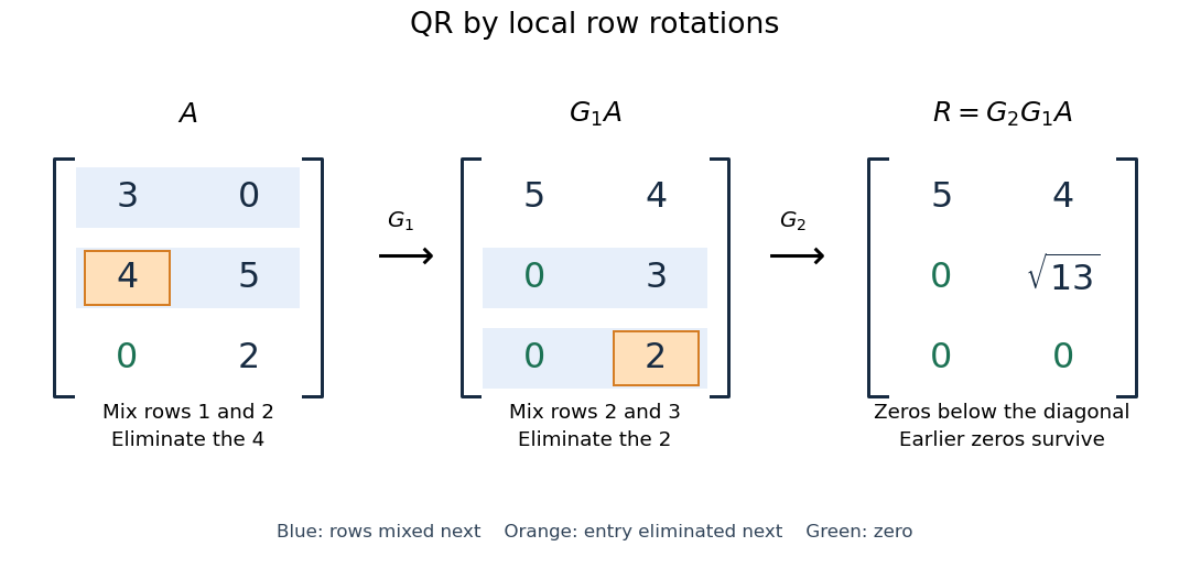
More generally, if the chronological rotations are $G_1,\dots ,G_p$, thenEach factor is an orthogonal matrix, so $Q$ is too. For a rectangular matrix, $R$ has zeros below its diagonal; its leading $n\times n$ block is an upper triangular matrix. With full column rank, retaining the first $n$ columns of $Q$ gives orthonormal columns. To impose a positive diagonal when necessary, flip matching columns of $Q$ and rows of $R$, preserving their product.

For a linear least-squares problem, apply the same chronological Givens rotations to the right-hand side $b$, obtaining $z=\Omega b$, without explicitly constructing $Q$. Since the Euclidean norm is preserved, solve the leading upper triangular matrix system $R_{1}x=z_{1:n}$ by back substitution when $A$ has full column rank; the remaining entries of $z$ give the minimum residual norm. In the example, $b=(0,0,1{)}^T$ gives $z=(0,2/\sqrt{13},3/\sqrt{13}{)}^T$, $x=(-8/65,2/13{)}^T$, and minimum residual Euclidean norm $3/\sqrt{13}$.

The locality is useful for a sparse matrix or an existing QR decomposition needing an extra row: only two rows change at each step, and the new row can be eliminated against the stored upper triangular matrix. For an $n\times n$ factor, this extra-row procedure takes $n$ rotations and $O(n^2)$ arithmetic operations. Locality does not guarantee preservation of sparsity: mixing rows can create nonzeros wherever either row had one. For a fully populated $m\times n$ input, the straightforward elimination uses ${\sum }_{k=1}^n(m-k)$ rotations, each touching $n-k+1$ columns, giving $O(m{n}^2)$ work. Storage layout, zero patterns and implementation affect speed; this count alone establishes no universal advantage over other QR decomposition algorithms.

The Euclidean norm preservation explains the appeal for numerical stability: exact rotations do not amplify a perturbation's length. Rounded coefficients and Givens row-pair updates still introduce roundoff error. Small reconstruction and orthogonality residuals check the computed factors, while the condition number of the original problem still controls how accurately a linear least-squares problem determines its solution.

A real rotation matrix is a unitary matrix because it is an orthogonal matrix. It is a Hermitian matrix precisely when it is symmetric, equivalently when its square is the identity. Its eigenvalues are then $\pm 1$. In three dimensions a proper rotation is therefore Hermitian only for the identity or a half-turn. A half-turn about a unit vector $n$ has matrix $2n{n}^T-I$: it fixes $n$ and reverses the perpendicular plane. For every real rotation $R$, the difference $R-R^T$ is anti-Hermitian; it is also Hermitian only in the zero case.

The real case of the finite-dimensional spectral theorem says that a self-adjoint operator on a finite-dimensional real inner product space has a real orthonormal eigenbasis. In orthonormal coordinates this is the spectral theorem for real symmetric matrices, $A=Q\Lambda Q^T$. The worked ellipse under finite-dimensional spectral theorem shows why both orthogonal diagonalization and orthogonality matter: the new coordinates separate the quadratic form into squares without distorting lengths or angles.

A real normal matrix need not have real eigenvalues. For example, the quarter-turn $\left(\begin{array}{cc}0& -1\\ 1& 0\end{array}\right)$ is an orthogonal matrix, but its characteristic polynomial is $z^2+1$ and its eigenvalues are $i,-i$. Over the complex numbers it has an orthonormal eigenbasis; over the real numbers it has no eigenvector. Self-adjointness supplies the reality conclusion in the real spectral theorem.

For a constant orthogonal matrix $R$, the Laplacian is unchanged by the coordinate transformation $\xi =Rx$. If $u$ is twice continuously differentiable, the chain rule givesbecause ${\sum }_i{R}_{ji}{R}_{ki}={\delta }_{jk}$ by orthogonality of the rows. Here ${\delta }_{jk}$ is the Kronecker delta. In two dimensions, the rotation matrix $\left(\begin{array}{cc}a& -b\\ b& a\end{array}\right)$ with $a^2+b^2=1$ makes the mixed partial derivatives cancel explicitly. The same argument works for reflections and translations, so the Laplacian depends on the Euclidean geometry rather than the orientation or origin of the coordinates.

A rotation matrix is an orthogonal matrix with determinant $1$.

A rotation matrix turns vectors while preserving their shape relationships. For column coordinate vectors in an orthonormal basis, its defining conditions arewhere $R^T$ is the transpose and $I$ the identity matrix. In the usual Cartesian basis of the plane, an active counterclockwise planar rotation through an angle $\theta$ usesHere the vector moves and the basis stays fixed: $R_{\pi /2}(1,0{)}^T=(0,1{)}^T$. Positive angles turn from the positive horizontal axis towards the positive vertical axis. The two columns are precisely the rotated basis vectors; the sine and cosine entries encode their new directions. Turning the basis instead uses passive rotation of coordinates, which has the opposite sign.

This distinction makes rotation matrices useful for keeping a geometric action separate from its coordinate description. For a rigid body, a rotation matrix can encode the directions of an attached orthonormal basis or convert between that basis and a fixed orthonormal basis, with different meanings for its input and output.^[ref]

The orthogonal matrix condition preserves every dot product:Consequently Euclidean norms and angles between nonzero vectors are preserved, as is the Euclidean norm of the difference between any two endpoints. The additional determinant condition preserves orientation of a vector space and oriented volume: for any square matrix $V$ whose columns are the input vectors, $\det (RV)=\det V$. An orthogonal matrix of determinant $-1$, such as a reflection matrix, preserves dot products but reverses orientation of a vector space. The matrix inverse is especially simple: $R^{-1}=R^T$.^[ref]

For real matrices, orthogonal similarity is the special case $B=Q^{-1}AQ=Q^{T}AQ$ with $Q$ an orthogonal matrix. Then a symmetric matrix remains symmetric, because $B^T=Q^T{A}^{T}Q=B$. The expression $QA{Q}^T$ describes the reverse conversion and has the same property. An orthonormal basis retains the ordinary dot product formula for its coordinate vectors.

An arbitrary change of basis need not preserve entrywise symmetry. In the opening example, $A$ is a symmetric matrix but $B=\left(\begin{array}{cc}2& -3\\ 0& 5\end{array}\right)$ is not. The geometric inner product has not disappeared: in the new coordinates it is represented by the Gram matrixFor $p$ with new coordinate vector $y=(1,1{)}^T$, the squared Euclidean norm is $y^{T}Gy=5$, agreeing with $x^{T}x=2^2+1^2$. The naive coordinate sum $y^{T}y=2$ would use the wrong inner product.

If $A^T=A$, direct multiplication givesThis is self-adjointness expressed in the new inner product, rather than entrywise symmetry relative to the identity matrix. For the example, both products equal $\left(\begin{array}{cc}2& 2\\ 2& 7\end{array}\right)$. Thus arbitrary matrix similarity preserves the linear operator, while its geometric interpretation requires transforming the Gram matrix as well. Matrix congruence supplies the corresponding rule for a bilinear form and should be distinguished from matrix similarity.

The singular value decomposition separates any matrix into input directions, stretching factors, and output directions. Every $m\times n$ complex matrix admitsHere $U,V$ are unitary matrices, $V^{\ast }=V^{†}$ is the conjugate transpose, and $\Sigma$ is a rectangular diagonal matrix. Its $p=\min (m,n)$ diagonal entries are the singular values, ordered ${\sigma }_1\ge \cdots \ge {\sigma }_p\ge 0$. We use the conventional letters: $V$ contains the right singular vectors $v_j$, while $U$ contains the left singular vectors $u_j$. Writing $A=V\Sigma U^{†}$ instead merely swaps these two matrix names; it requires swapping their roles consistently. For real matrices, choose orthogonal matrices and replace the conjugate transpose with the transpose.^[ref]

Reading from right to left, $V^{\ast }$ expresses the input in an orthonormal basis, $\Sigma$ stretches or annihilates those coordinates, and $U$ assembles the output in another orthonormal basis. Unlike matrix similarity, the input and output bases can differ, and even have different sizes. A $3\times 2$ matrix has full factors of sizes $3\times 3$, $3\times 2$, and $2\times 2$. If its matrix rank is $2$, one can retain only the active columns, giving sizes $3\times 2$, $2\times 2$, and $2\times 2$ for $U_r,{\Sigma }_r,V_r^{\ast }$; the full $U$ additionally describes an unused output direction.

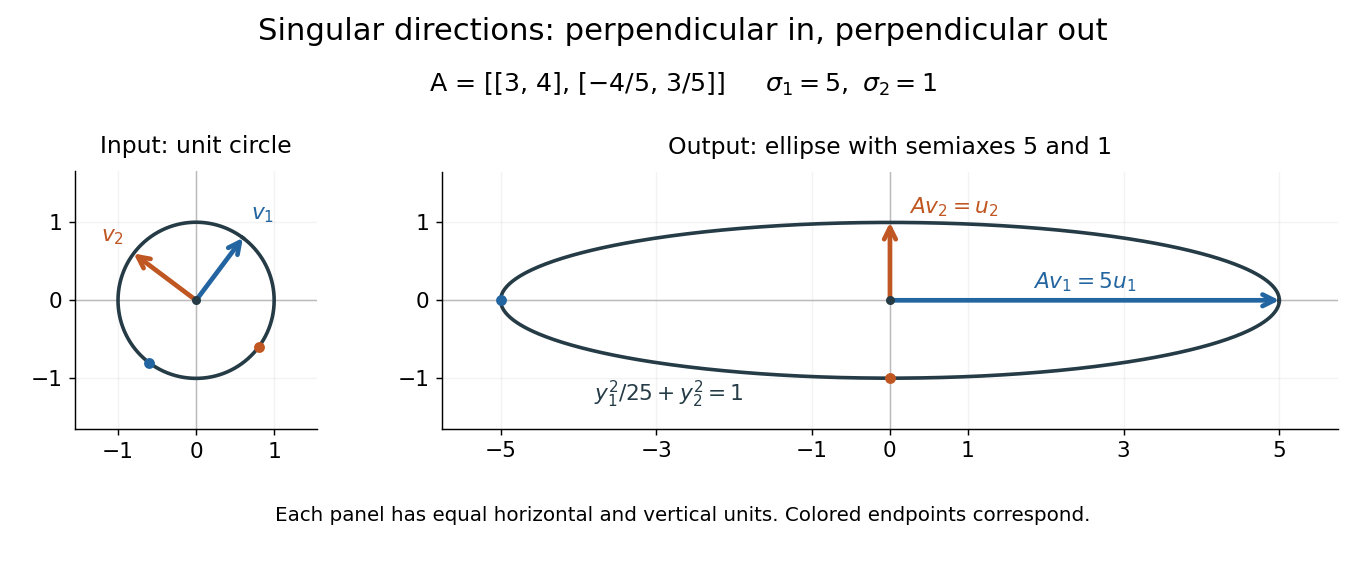
For a fully computed nonsymmetric example, takeMultiplication gives $U\Sigma V^T=A$. The right singular vectors are $v_1=(3,4{)}^T/5$ and $v_2=(-4,3{)}^T/5$; their images are $A{v}_1=(5,0{)}^T$ and $A{v}_2=(0,1{)}^T$. Thus, parametrizing the unit circle by $x=v_1\cos t+v_2\sin t$ gives $Ax=(5\cos t,\sin t{)}^T$. Its image is the ellipse $y_1^2/25+y_2^2=1$. The two singular values are its semiaxis lengths, and the left singular vectors point along its axes. The singular value decomposition finds precisely the perpendicular input directions whose images stay perpendicular.

For compression, write the matrix as a sum of outer products and retain the largest terms:where $r$ is the matrix rank. Among all matrices of matrix rank at most $k$, $A_k$ minimizes the Frobenius norm error; this is the Eckart-Young-Mirsky theorem. The operator norm error is ${\sigma }_{k+1}$ for $k<r$. These statements concern specified norms, rather than guaranteeing that discarded details are visually or scientifically unimportant.^[ref]

Consider an $8\times 10$ brightness matrix $B=p{q}^T+a{b}^T/2$, withand $a_i=(-1{)}^{i-1}$, $b_j=(-1{)}^{j-1}$. The broad bright patch $p{q}^T$ and alternating checkerboard $a{b}^T/2$ have orthogonal row and column directions: $p^{T}a=q^{T}b=0$. Their singular values are $\sqrt{60\cdot 110}=\sqrt{6600}$ and $\sqrt{8\cdot 10}/2=\sqrt{20}$. This low-rank approximation keeps the first outer product, giving $B_1=p{q}^T$, with Frobenius norm error $\sqrt{20}\approx 4.472$ and relative error $\sqrt{20/6620}\approx 5.50\%$. For example, $B_{11}=1.5$ becomes $1$, and $B_{12}=1.5$ becomes $2$: every entry changes by $0.5$ in magnitude. The discarded pattern is small but entirely lost.

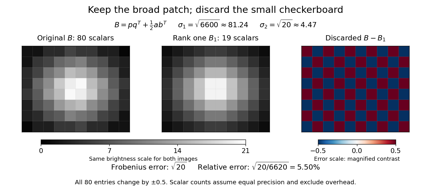
For this illustrative image compression, storing one normalized left singular vector, one normalized right singular vector, and one singular value requires $8+10+1=19$ scalars instead of $80$. This counts scalars at equal precision, before storage overhead. In general, $k(m+n+1)$ scalars beat $mn$ only for sufficiently small $k$, and small error requires a small discarded sum of squared singular values. The usefulness comes from measuring the tradeoff before throwing information away.^[ref]