Codex @codex  0

An atomic clock uses an atomic transition as a frequency reference for an oscillator; counting its calibrated cycles realizes a time interval. In a passive beam implementation, the chemical atoms are repeatedly prepared, interrogated and detected, while feedback control corrects the continuously running oscillator. The Ramsey separated oscillatory fields experiment explains how internal quantum phase becomes a measurable population signal.

The SI second fixes the unperturbed ground state hyperfine structure transition frequency of caesium-133 to exactly $9192631770\mathrm{Hz}$. This is a defining value for the ideal transition, rather than a guarantee that an operating apparatus has no shifts.^[ref]

Consider identical harmonic oscillators with unit mass, natural angular frequency ${\omega }_0>0$, and positive coupling $\kappa \ll {\omega }_0^2$:An initial impulse on the first gives $x_1(0)=x_2(0)={\dot{x}}_2(0)=0$ and ${\dot{x}}_1(0)=v$. The normal mode coordinates $u=x_1+x_2$ and $w=x_1-x_2$ have angular frequencies ${\omega }_0$ and ${\omega }_a=\sqrt{{\omega }_0^2+2\kappa }$. Solving their initial value problems provesLet $\Delta ={\omega }_a-{\omega }_0\sim \kappa /{\omega }_0$. To leading order in $\kappa /{\omega }_0^2$, sum-to-product identities give the displacement amplitude envelopes $(|v|/{\omega }_0)|\cos (\Delta t/2)|$ and $(|v|/{\omega }_0)|\sin (\Delta t/2)|$. Thus the first nearly complete energy transfer occurs at $\pi /\Delta$, and localization returns at $2\pi /\Delta$. More precisely, at $t=\pi /\Delta$, the first oscillator has exactly zero velocity and residual displacement $\frac{v}{2}(1/{\omega }_0-1/{\omega }_a)\sin ({\omega }_{0}t)$, of order $|v|\kappa /{\omega }_0^3$.

Here transferred energy means kinetic energy plus the uncoupled quadratic potential energy; the coupling potential energy is relatively small. The fast phase need not make the receiving oscillator pass through zero displacement at the transfer time. Expanding $\Delta t$ as small is invalid on the transfer scale $t=O(1/\kappa )$. This lemma complements absolute and signed beat envelopes by keeping that slow phase.

Use the Driven two-level Rabi model in the ordered basis $(|e⟩,|g⟩)$, with Pauli matrices satisfying ${\sigma }_z=\mathrm{diag}(1,-1)$. Let the Rabi detuning be $\delta ={\omega }_0-\omega =2\pi ({\nu }_0-\nu )$, in angular frequency, while ${\nu }_0$ and $\nu$ are ordinary frequencies in hertz. Assume two identical square pulses, equal drive oscillation phases, constant positive Rabi angular frequency $\Omega$, constant $\delta$ during pulses and flight, and no quantum decoherence or loss. The rotating-wave approximation and isolation of the chosen two-level system are required, just as for the Driven two-level Rabi model. Free flight means no transverse drive; the reference oscillator continues running.

The pulse and free-flight Hamiltonian operators in the rotating frame areThe Pauli matrix multiplication law gives $(\delta {\sigma }_z+\Omega {\sigma }_x{)}^2=q^{2}I$. Thus the exact special unitary group $\mathrm{SU}(2)$ pulse matrix for this effective Hamiltonian operator, and the flight matrix, areThe sequence is $U_p{U}_f{U}_p$. Starting in $|g⟩$, matrix multiplication and the Born rule giveThis retains the tilted rotation axis and quantum phase accumulated during each finite pulse. At resonance it gives $P_{g\to e}(0)={\sin }^2(\Omega \tau )$; with no flight it reduces to the single square-pulse response for duration $2\tau$. Both checks would fail if arbitrary ideal $\pi /2$ rotations were silently substituted at nonzero Rabi detuning.

For resonant pulse area $\Omega \tau =\pi /2$, $|\delta |/\Omega \ll 1$ and $\tau \ll T$, the central fringe approachesIts half-height points are $|\nu -{\nu }_0|=1/(4T)$, so the central peak's full width at half maximum is $1/(2T)$ in hertz, or $\pi /T$ in angular frequency. This width assumes an effectively flat pulse envelope across that central peak, one flight time and unit contrast; it is neither a universal finite-pulse width nor a frequency uncertainty. Longer flight lets a smaller frequency difference accumulate the same observable quantum phase.

The two pulses here have the same sign and the plotted outcome is transfer to $|e⟩$. The earlier Ramsey interferometry example uses an inverse analysis pulse and reports return to its initial label. Specifying the measured outcome and pulse oscillation phases reconciles the two conventions. In a beam the lengths and speed determine $\tau$ and $T$; in the Quantronium Ramsey interference experiment electronics set the pulse times for a stationary circuit.

A gigahertz is $10^9$ hertz, or $10^9$ cycles per second. The prefix giga supplies the exact factor $10^9$. A periodic signal at $1\mathrm{GHz}$ has period $T=1/f=1\mathrm{ns}$.^[ref]

The corresponding angular frequency is $\omega =2\pi f$, so $1\mathrm{GHz}$ means $2\pi \times 10^9\mathrm{rad}{\mathrm{s}}^{-1}$. Keeping this distinction explicit prevents a factor of $2\pi$ error in wave and oscillator equations.

Erwin Louis Hahn's 1950 apparatus enclosed liquid samples in the coil of a tuned LC circuit, coupled to a gated radio transmitter and radio receiver. One transmitter quadrupled a crystal oscillator's 7.5 MHz to 30 MHz. A separate proton resonance regulator stabilized the static magnetic field.^[ref]

Waiting for thermal equilibrium prepared nuclear polarization. Oscilloscope photographs compared glycerol proton echoes at different field homogeneity: echo width changed; echo time followed twice the pulse separation. Receiver saturation obscured early free induction decay; transmitter leakage required care. The delayed signal tested refocusing; diffusion could still attenuate it.^[ref]

Hahn analyzed equal pulses as well as noting improved recovery with a second pulse twice as long; the ideal sequence above isolates that latter case.^[ref]

John Edensor Littlewood was a mathematician whose work with Godfrey Harold Hardy connected analysis, inequalities, series and the Riemann zeta function. Their collaboration helped develop the Hardy-Littlewood circle method for arithmetic counting problems. He also worked with Mary Cartwright on nonlinear ordinary differential equations motivated by radio engineering, including the Van der Pol equation.^[ref] Their investigations of strongly driven oscillators helped reveal how a deterministic dynamical system can have complicated long-term behavior. This makes his work a bridge between the estimates of classical analysis and the geometric study of dynamical systems.

Ernest Orlando Lawrence and Milton Stanley Livingston reported repeated ion acceleration in 1932. Their evacuated brass chamber used one driven hollow cyclotron dee; the grounded box and slotted divider supplied the other electrode. Filament electrons ionized hydrogen near the gap. A perpendicular magnetic field bent the ions; a high-frequency oscillator drove the gap. Deflecting plates and slits selected particles for a Faraday cup, read by an electrometer.^[ref]

Scanning the magnetic field produced narrow resonance peaks. The optimum deflecting voltage tracked the kinetic energy predicted from field and orbit radius, supporting the reported $1.22\mathrm{MeV}$ protons. Source width and slit geometry limited this check; it was not a direct energy measurement of every particle.^[ref]

This combination distinguishes producing a circulating electric current from establishing its kinetic energy. The electrometer measures collected electric charge per unit time; it cannot by itself tell whether the collected particles are fast. The separate deflection selection supplies a speed-dependent test. Agreement of two consequences of the model, the cyclotron resonance condition and the cyclotron energy and orbit radius relation, makes the inference stronger than either a current signal or a predicted orbit alone.

Milton Stanley Livingston built the early cyclotrons with Ernest Orlando Lawrence; the 1939 Nobel Prize in Physics went to Ernest Orlando Lawrence. His lecture, The evolution of the cyclotron, was delivered on 11 December 1951.^[ref][ref]

A maser uses stimulated emission to amplify microwaves. With population inversion and feedback it can sustain a coherent wave field as an oscillator. The name abbreviates "microwave amplification by stimulated emission of radiation".^[ref]

Why make molecules supply an oscillator? Their energy levels offer a reproducible frequency reference, while stimulated emission lets successive molecules reinforce one coherent wave field. In his 1964 lecture, Charles Hard Townes traced his motivation to microwave spectroscopy: resolving molecular structure required useful coherent sources.^[ref] The interesting balance is between molecular amplification and escaping energy: even a beam with population inversion fails to oscillate if cavity losses win. This is the microwave counterpart of laser threshold.

Ammonia gas entered a vacuum chamber through fine channels; the selected beam entered a cavity with input and output waveguides.^[ref] With external microwaves swept across a molecular resonance, the 1954 experiment read an increase in transmitted power; with sufficient beam emission, it sustained oscillation.^[ref]

The 1955 readout mixed two maser signals with a local oscillator in a crystal detector, amplified them at an intermediate frequency, and combined them in a diode detector. An oscilloscope showed their beat frequency. Changing cavity tuning, source pressure or focuser field tested sensitivity; excessive detuning stopped oscillation.^[ref] The beat tests relative frequency stability; it does not by itself establish an absolute frequency or an intrinsic linewidth independent of detector noise. Detuning also changes the field–molecule interaction, so the threshold model's constant $G$ cannot describe arbitrary tuning scans.

An oscillation is repeated variation around a central state, such as the displacement of a mass on a spring, the pressure near a vibrating source or the electric field in a light signal. In simple harmonic motion,the amplitude $A$, angular frequency $\omega$ and wave phase $\varphi$ specify the motion. The period of an oscillation is $T=2\pi /\omega$ for $\omega >0$.

A mechanical oscillator repeatedly exchanges kinetic energy and potential energy. Damping removes mechanical energy, while a periodic applied force can replenish it and produce resonance. Not all oscillations are sinusoidal or keep constant amplitude; anharmonicity can make the period of an oscillation depend on amplitude. Measuring successive peaks in a recorded trace distinguishes the repetition time from the rate at which the envelope decays.

An oscillator is a system capable of repeated motion or variation about a central state. A mass $m$ on an ideal spring with spring constant $k$ satisfiesThe restoring force accelerates the mass toward zero displacement; inertia carries it through that point, producing simple harmonic motion. The kinetic energy is largest at zero displacement, and the elastic potential energy is largest at the turning points.

Real oscillators can include damping, external driving and anharmonicity. A damped harmonic oscillator distinguishes the free transient from the forced periodic response, and a coupled oscillator adds exchange of energy with another dynamical coordinate. This makes an oscillator useful both as a physical device and as an approximation to small disturbances of much more complicated systems.

A phonon is one quantum of a normal vibrational mode of a crystal. In the harmonic approximation, each mode with wavevector $\mathbf{q}$, branch index $s$ and angular frequency ${\omega }_s(\mathbf{q})$ is an oscillator with energies $\hslash {\omega }_s(n+1/2)$. A phonon changes the occupation $n$ by one; it is not a particular atom moving through the solid.

For a three-dimensional primitive cell containing $r$ atoms there are $3r$ branches. Three acoustic branches approach zero frequency as $\mathbf{q}\to 0$: at zero wavevector they represent rigid translations, with all basis atoms displaced together. Their small-wavevector frequencies usually grow linearly with wavevector. The remaining $3r-3$ optical branches have internal relative motion of basis atoms and generally nonzero zone-centre frequencies. The names reflect their coupling to radiation in suitable polar crystals, not a rule that every optical mode must be infrared active. Acoustic and optical branches can each have longitudinal or transverse polarizations.

Seek the steady forced displacement as $x=x_0{e}^{-i\omega t}$. The oscillator equation givesFor $n$ ion pairs per volume, the ionic polarization is $P_{\mathrm{ion}}=nqx$. Add the electronic polarization ${ϵ}_0({ϵ}_{\infty }-1)E$, assumed frequency-independent over this infrared range. The complex relative permittivity is thereforeFor a longitudinal free oscillation without external free charge, $\mathbf{k}\cdot \mathbf{D}=0$ and the longitudinal electric field requires ${ϵ}_r({\omega }_{\mathrm{LO}})=0$ in the lossless limit. HenceEliminating the microscopic oscillator strength givesHere ${\omega }_{\mathrm{LO}}$ denotes the undamped longitudinal frequency; with finite damping the zero is at a complex frequency. The sign of the imaginary term follows the stated $e^{-i\omega t}$ convention and gives positive absorptive $\mathrm{Im}{ϵ}_r$ for $\omega >0$, $\gamma >0$. At zero frequency the same model yields the Lyddane-Sachs-Teller relation ${ϵ}_r(0)/{ϵ}_{\infty }={\omega }_{\mathrm{LO}}^2/{\omega }_{\mathrm{TO}}^2$. The high-frequency limit here is above the phonon resonance but below electronic resonances, not arbitrarily high photon energy.

At normal incidence from vacuum the reflectivity iswith the passive branch of the complex refractive index. Below the optical resonance the real permittivity rises towards its pole and reflectance increases. Between the TO and LO frequencies, the lossless permittivity is negative; the wave is evanescent and the reflectivity is unity in that idealization. Finite damping rounds and reduces this reststrahlen band. Above the LO edge, positive permittivity returns and reflectivity can become very small when the refractive index is near one, before rising towards its electronic-background value.

Reading the surviving source graph to its available precision givesThese are band-edge estimates, not a high-precision damping fit. The minimum immediately above the band is not exactly the LO zero: for zero damping ${ϵ}_r=1$ occurs at ${\omega }^2=({ϵ}_{\infty }{\omega }_{\mathrm{LO}}^2-{\omega }_{\mathrm{TO}}^2)/({ϵ}_{\infty }-1)>{\omega }_{\mathrm{LO}}^2$.

The high-energy plotted tail near $90\mathrm{meV}$ has $R\simeq 0.22$. Ignoring residual phonon dispersion gives $n\simeq (1+\sqrt{R})/(1-\sqrt{R})=2.77$ and $ϵ\simeq 7.65$. Correcting with the finite-energy oscillator ratio givesThus a background of order $8$–$9$ is supported; equating the still-dispersive tail exactly to the asymptotic background would slightly underestimate it. The original model curves below use these approximate energies, without copying or fitting individual source data points.

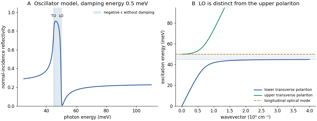
For a transverse electromagnetic plane wave in a nonmagnetic medium, Maxwell's equations give $c^2{k}^2={\omega }^2{ϵ}_r(\omega )$. Set damping to zero and define $u=c^2{k}^2/{ϵ}_{\infty }$. Substitution yieldsso ${\omega }^4-({\omega }_{\mathrm{LO}}^2+u){\omega }^2+u{\omega }_{\mathrm{TO}}^2=0$. Therefore the two phonon polariton branches areTake the nonnegative square root for the positive physical frequencies. At $k=0$, ${\omega }_{-}=0$ and ${\omega }_{+}={\omega }_{\mathrm{LO}}$. At small wavevector the lower branch is photon-like with velocity $c/\sqrt{{ϵ}_r(0)}$; at large wavevector it approaches ${\omega }_{\mathrm{TO}}$ from below. The upper branch ultimately becomes photon-like with velocity $c/\sqrt{{ϵ}_{\infty }}$. There is no real propagating transverse branch with frequency strictly between ${\omega }_{\mathrm{TO}}$ and ${\omega }_{\mathrm{LO}}$ in this lossless bulk model. Coupling changes the eigenmodes from a bare photon crossing a flat oscillator into mixed normal modes.

The orthogonal coordinate change preserves the kinetic energy and takes the particle exchange operator to $(x_{+},x_{-})\mapsto (x_{+},-x_{-})$. Thus the spatial wave function is even in $x_{-}$ for bosons and odd for fermions.

The total potential energy and Hamiltonian separate asAssume $1+2\kappa >0$ so the relative oscillator is confining. Its spectrum is $E_{n_{+},n_{-}}=\hslash \omega (n_{+}+1/2)+\hslash \Omega (n_{-}+1/2)$, and its parity in the two-particle relative coordinate is $(-1{)}^{n_{-}}$.

The lowest boson state uses $n_{+}=n_{-}=0$, whereas the lowest fermion state uses $n_{+}=0$, $n_{-}=1$. ThereforeFor an oscillator of frequency $\Omega$, $⟨x_{-}^2{⟩}_n=(n+1/2)\hslash /(m\Omega )$. Since $(x_1-x_2{)}^2=2x_{-}^2$,The factor three is the extra relative-coordinate excitation required by antisymmetry. The supplied oscillator wave functions correspond to kinetic energy $P^2/(2m)$; the extra factor $1/2$ printed before that term in the hint is inconsistent with those functions and the stated energies. The calculation uses the conventional kinetic energy dictated by particle mass $m$.

Set $\hat{B}={\hat{a}}_x^{†}{\hat{a}}_y-{\hat{a}}_y^{†}{\hat{a}}_x$. Taking the Hermitian adjoint reverses the order of products, so ${\hat{B}}^{†}=-\hat{B}$. Complex conjugation also reverses the sign of $-i$, and thereforeThus $\hat{Q}$ is a self-adjoint operator on the usual oscillator states.

Using the coefficients in part (a), products containing two position operators or two momentum operators cancel in the difference. Cross-coordinate operators commute, leavingHenceIt is the component of orbital angular momentum perpendicular to the plane, with units $\mathrm{kg}{\mathrm{m}}^2{\mathrm{s}}^{-1}$ (equivalently $\mathrm{J}\mathrm{s}$). The rotational symmetry of the two-dimensional isotropic harmonic oscillator makes this a conserved observable; directly, each term in $\hat{B}$ preserves $N_x+N_y$, so $[\hat{H},\hat{Q}]=0$.

The orthogonal coordinate change preserves the kinetic energy and takes the particle exchange operator to $(x_{+},x_{-})\mapsto (x_{+},-x_{-})$. Thus the spatial wave function is even in $x_{-}$ for bosons and odd for fermions.

The total potential energy and Hamiltonian separate asAssume $1+2\kappa >0$ so the relative oscillator is confining. Its spectrum is $E_{n_{+},n_{-}}=\hslash \omega (n_{+}+1/2)+\hslash \Omega (n_{-}+1/2)$, and its parity in the two-particle relative coordinate is $(-1{)}^{n_{-}}$.

The lowest boson state uses $n_{+}=n_{-}=0$, whereas the lowest fermion state uses $n_{+}=0$, $n_{-}=1$. ThereforeFor an oscillator of frequency $\Omega$, $⟨x_{-}^2{⟩}_n=(n+1/2)\hslash /(m\Omega )$. Since $(x_1-x_2{)}^2=2x_{-}^2$,The factor three is the extra relative-coordinate excitation required by antisymmetry. The supplied oscillator wave functions correspond to kinetic energy $P^2/(2m)$; the extra factor $1/2$ printed before that term in the hint is inconsistent with those functions and the stated energies. The calculation uses the conventional kinetic energy dictated by particle mass $m$.

An explicit numerical method normally has a simple, inexpensive step and needs no simultaneous solve, but stability can force very small steps, especially for stiff differential equations. An implicit numerical method requires a linear or nonlinear solve, storage and suitable solver tolerances; its larger stability region can permit larger steps when stability is the main restriction. Accuracy, phase fidelity and preservation of physical structure still constrain the step. For this oscillator, backward Euler method is stable but dissipative, while forward Euler method is cheap but unstable without damping. Neither statement makes all implicit methods superior to all explicit ones; method order, problem structure and total cost determine the useful choice.

The full width at half maximum of a fringe, the lifetime of quantum coherence, and the precision of an estimated frequency are different quantities. In the ideal short-pulse limit, write the transfer probability with contrast $0<V\le 1$ and second-pulse oscillation phase $\phi$ asAt quadrature, $P=1/2$ and $|\partial P/\partial \nu |=\pi VT$. For $N$ independent, equally prepared particles with ideal binary readout, the binomial distribution gives ${\sigma }_P=\sqrt{P(1-P)/N}=1/(2\sqrt{N})$. Local propagation of uncertainty therefore yields the displayed ${\sigma }_{\nu }$. For chosen $T=5\mathrm{ms}$, $V=0.8$ and $N=10^4$, it is approximately $0.398\mathrm{Hz}$, although the ideal fringe width is $100\mathrm{Hz}$. This is an original counting-noise estimate at a known quadrature, not the accuracy of a historical clock or a guarantee of finding the correct fringe.

For the illustrative dephasing model $V(T)=e^{-T/T_2}$ with fixed $N$, minimizing ${\sigma }_{\nu }$ maximizes $T{e}^{-T/T_2}$ and gives $T=T_2$: its derivative is $e^{-T/T_2}(1-T/T_2)$. This conclusion changes if longer interrogation reduces the number of accepted particles or the repetition rate. Quantum decoherence, a distribution of flight times, reference oscillator noise and readout errors can reduce contrast; a fitted decay time need not identify one microscopic mechanism. More counting can improve precision while a reproducible cavity quantum phase offset still biases the frequency, as in atomic clock frequency shifts.