Direct matrix multiplication gives the multiplication tableTogether with acting as the identity, this shows that the product of any two real linear combinations is again a real linear combination. Thus is closed under multiplication. It is the complex matrix representation of quaternions.
Its general element has the formIf this matrix is zero, real and imaginary parts of its first row give . Hence are linearly independent over and form a basis:Put . Since distinct imaginary units anticommute, the mixed terms in cancel, leaving . Scalars commute with , soThe reversed product is the same. The coefficient is strictly positive for every nonzero element. ConsequentlyThis also identifies as a real noncommutative division algebra, not as the full algebra of complex two-by-two matrices.
A group automorphism is a bijective group homomorphism from to itself. The multiplication in is composition: . Composition is associative, the identity map is the identity element, and each inverse bijection is again a homomorphism, so these maps form the automorphism group.
For conjugation by , multiplication is preserved becauseConjugation by is its inverse, so is an group automorphism. MoreoverHence is a homomorphism, with image the inner automorphisms. Its group homomorphism kernel is the group center of , since is the identity precisely when for every .
Every uniformly continuous function on is bounded. Choose the tolerance for and an integer with . The finitely many centers , , cover the interval by cells of radius . For each , one center satisfies . Thus . This is the uniformly continuous function on a totally bounded set is bounded argument; closedness of the interval is unnecessary.
The reciprocal function is not uniformly continuous on . It is unbounded, already contradicting the preceding result. Directly, and have distance tending to zero while .
The oscillating function is not uniformly continuous either, despite being bounded. TakeTheir distance tends to zero, but their function values are and . The fixed output gap of two contradicts the uniform-continuity condition, for example with .
Suppose the union has a separation into disjoint, nonempty, relatively open subsets. Each connected must lie entirely in one of them: otherwise its intersections with and would separate in its subspace topology. In particular lies on one side, say . Every other intersects , so it cannot lie in and must also lie in . Then , contradicting . The union is connected. This is the connected union with a connected hub argument.
For path-connectedness, take any and . Choose and . There is a path from to inside , a path from to inside , and a path from to inside . Concatenate the three paths on successive thirds of . They agree at the joining points, so the resulting map is continuous and remains in . The union is path-connected. There need not be a single point common to all the subsets.
Use the causal Green function: it vanishes before the forcing time . For it solves the homogeneous equation, is continuous at with value zero, and has first-derivative jump one. These conditions giveIndeed the right derivative at the forcing time is one and the left derivative is zero, so distributionally. If , use the continuous limit on its causal support.
For , differentiating the integral solution givesBoth initial values vanish and . This verifies the requested representation and its sign. The formula similarly gives .
In SI units, the sourced Maxwell equations areTake the divergence of the last equation. The divergence of a curl vanishes; using the first equation gives the necessary local conservation lawFor sources supported in a fixed region, integrate over a containing surface where the current vanishes. The divergence theorem givesThus the total charge is constant. For each component of the electric dipole moment, integration by parts givesThe surface term again vanishes, soSmooth compact support suffices for these manipulations; equivalently one may integrate the charge continuity equation over all space and use the fixed support to identify the integrals with those over .
Set , and . In Alice's inertial coordinates the departure, turn and return events are , and . Alice's worldline is vertical; Bob's consists of two straight timelike segments of slopes , joined by the short turnaround. Equal speeds and the same endpoints give equal coordinate durations on the two legs.
The Minkowski proper-time element for Bob is , while Alice at rest has . Integrating on both legs givesAcceleration itself need not cause a large direct change in the clock rate. Its role is to make Bob change inertial frames and reunite with Alice, so the two worldlines have different proper lengths between the same events.
To describe Bob's assignment of Alice's age, apply relativity of simultaneity to lines of equal coordinate time in his instantaneous inertial frames. At the turn the outbound line is ; it intersects Alice at . The inbound line is and intersects her at . Thus the negligibly short change of rest frame advances Bob's assigned Alice age by . On each inertial leg he assigns Alice an aging rate per unit of his own proper time, but the frame dependence expressed by relativity of simultaneity removes the apparent symmetric-time-dilation paradox.
If “sees” means clocks read from received light, there is no instantaneous jump in Alice's displayed age. A light signal received at Bob's event was emitted from Alice at . On the outbound leg ; on the inbound leg . Consequently the observed aging rates per Bob proper time areHe receives slowly running, redshifted clock signals on the outward leg and rapidly running, blueshifted signals on the return. Integrating both rates over the equal proper durations gives total received Alice aging , with the two expressions continuous at the turn.
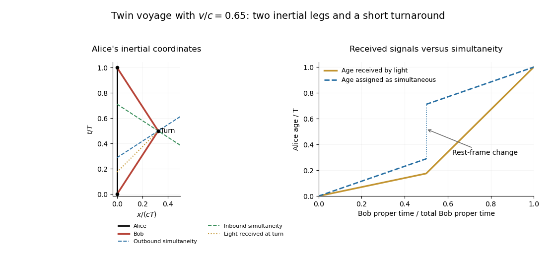
Twin voyage: inertial worldlines, turnaround simultaneity lines, and Alice ages assigned or optically received by Bob
. Details. 
The diagram distinguishes the reassignment due to relativity of simultaneity from the continuous optical observation; both descriptions give the same ages when the twins meet again.
The intended dynamical assumption is steady inviscid Euler flow of constant density, with conservative body-force potential . Its equation is . The vector identitythen givesWith no body force take . Taking the scalar product with yields , so the Bernoulli function is constant along streamlines, though not necessarily the same constant on different streamlines.
Choose the planar streamfunction convention . Then with , andIf locally , comparison with giveson the nonstagnant part of that flow. It extends to isolated stagnation points by continuity. Where the streamfunction is constant on an entire open region, cancellation of its zero gradient alone imposes no derivative condition on an arbitrarily extended .
Steadiness and incompressibility alone, without the inviscid dynamical assumption, do not imply the stated identity. In a steady Newtonian viscous flow the correct form has . For example, a pressure-driven planar Poiseuille flow has a nonzero streamwise pressure gradient balanced by viscosity, while has no streamwise component. This identifies the required qualification of the printed premise.
In a finite two-person zero-sum game the row player chooses , the column player chooses , and the row player receives while the column player receives . The row player maximizes that payoff and the column player minimizes it. Mixed strategies are probability vectors and , giving expected row payoff .
Against a fixed row mixture, the worst column is a pure column, so the row problem introduces its guaranteed payoff :Similarly the column player minimizes an upper guarantee :The values are unrestricted real variables; no positivity shift of the matrix is required.
To see the linear programming duality explicitly, introduce nonnegative multipliers for the first problem's payoff inequalities and multiplier for its normalization. Its upper-bound Lagrangian isThe supremum over free and nonnegative is finite precisely when and , and is then . Minimizing it gives the displayed column problem, proving that the programs are a dual pair.
A sufficient optimality certificate is a pair of probability vectors and a common value satisfyingEquivalently, both programs are feasible with equal values. Positive-probability rows then have and positive-probability columns have , the complementary slackness conditions. These conditions certify a saddle point and hence optimal mixed strategies for both players.
For a complex square matrix, define its determinant byThe cofactor is , where deletes row and column . The adjugate is the transposed cofactor matrix, .
The entry of is . For , expansion along column gives . For , this same sum is the determinant of the matrix obtained by replacing column by column : deleting the replaced column leaves all its cofactors unchanged. The new matrix has two equal columns, so its determinant is zero. ThusThis proof does not assume invertibility and therefore also covers singular matrices.
The cyclic matrix acts by . For each fourth root of unity , the vector satisfies , because . This supplies the four distinct eigenvalues and nonzero eigenvectors:Eigenvectors for distinct eigenvalues are linearly independent. Thus, with these columns in the indicated order,They form a basis over , so there are no other eigenvalues. Equivalently the characteristic polynomial is .
Let and . The precise presented group is , with and . It is abelian and has exactly the imposed additive relation and its integer multiples.
Change the integral basis to , . The change-of-basis determinant is , so these are a basis of the free abelian group. Explicitly, and . The relation generator becomes . ThereforeThe image of is nonzero, since is not an integer multiple of , but three times it vanishes. Thus has an element of exact order three. A free abelian group has no nonzero finite-order element, so is not free abelian.
For a Riemannian metric , write . Use the energy of a curve normalization compatible with the requested inequality:The Cauchy-Schwarz inequality here has the direct variance formEquality holds exactly when is constant almost everywhere, hence everywhere for a smooth curve. With the alternative energy of a curve convention containing a factor , the same assertion reads .
In the upper half-plane write , , and use . Let the endpoints be , , . ThenThe first equality requires throughout. Endpoint values force . The second equality requires the derivative of to have one sign, so is monotone. Conversely every smooth monotone positive with these endpoints attains this bound. Consequently the absolute length minimizers are precisely the vertical curves with monotone height, including a constant curve when , and the distance is .
For curves stationary for the energy of a curve, fixed-endpoint variations give the Euler–Lagrange equations for :Thus for a constant . Since , integration gives , hence . The second equation then becomes . ThereforeIt has constant hyperbolic speed, is one of the absolute length minimizers, and also has minimum energy of a curve .
Choose and put . The intersection is nonempty, closed and bounded in , hence compact. The continuous distance function attains a minimum at some . For its value is strictly greater than , while the value at is at most that at , namely . Thus this minimum on is a minimum on all of :The set itself need not be bounded; only the compact portion needed to find the nearest point is bounded.
Suppose two distinct minimizers have the same minimum distance from . Convexity puts their midpoint in . Expanding the Euclidean norm givescontradicting minimality. Therefore the nearest point is unique. Together with the preceding existence proof, this defines the metric projection onto a nonempty closed convex set.
Close the real-line contour by a positively oriented upper semicircle of radius , beyond every pole. The rational function is uniformly on that arc, and . Its arc integral is therefore and vanishes. The real integral is absolutely convergent, while no pole lies on it. The residue theorem givesOnly actual poles contribute; any removable zero of the denominator has zero residue. The same contour proof covers poles of any order.
For the particular denominator, the upper poles are and . They are simple, with residues and . Sincetheir sum isMultiplication by gives the real answer. The sine part of the real-line integral is zero by oddness, so
Fixed endpoint variations yield the Euler–Lagrange equationWhen is independent of , differentiation givesThis is the Beltrami identity. Denote the constant by when nonzero; for a general Lagrangian a zero constant is also possible.
The film area is . Suppressing its harmless positive factor , take . The Euler–Lagrange equation reduces toThe first integral is with . Hence and, using the differential equation without dividing by , . The positive solution obeying that first integral is . Equal endpoint radii force , givingThus every smooth positive stationary film in this axisymmetric class is a catenoid.
Put . The boundary equation is . The function tends to infinity at both endpoints of , andIts minimum occurs when . The function is strictly increasing, with derivative , and has limits and . It therefore has exactly one positive zero . At this point , so . This proves the catenoid existence threshold for equal rings:At equality there is one stationary solution and above it two. The equation describes candidates for an area minimum, not a guarantee that both branches minimize. The thinner-neck branch is unstable to suitable axisymmetric variations; topology-changing collapse can also compete with connected films. In particular two separate planar disks have area . The derived threshold concerns existence of the smooth annular stationary film; it does not exclude such disconnected competitors.
On a suitable dense domain of smooth rapidly decreasing wave functions, the canonical commutator is . Expanding the two ladder operators givesTheir sum and difference giveDirect multiplication, retaining the operator order, givesUsing identifies the Hamiltonian operator:For any admissible wave function, adjointness givesFor the conventional normalized state , this is the stated lower bound . For an unnormalized function the norm factor must be retained; rescaling a wave function cannot leave its unnormalized energy integral bounded below by a fixed positive number.
Equality holds exactly when . In position representation this equation is , whose normalized square-integrable solution isThis construction establishes existence of a state attaining the bound, and hence proves that it is the ground state.
The commutator implies . Repeatedly commuting through the product givesThese vectors are nonzero: the identity gives their norm squared by induction. ThereforeFor time-dependent stationary states multiply each spatial eigenfunction by .
In Cartesian coordinates the magnetic field is . Its divergence is , and all components of its curl vanish. Thus it satisfies the static vacuum magnetic equations and , with no electric current in the region.
Fix clockwise orientation as viewed from above, looking down the positive -axis. Its positive area normal is . The loop's external magnetic flux is thereforeWith the opposite normal its flux has the opposite sign. On the circle and clockwise line element is . The Lorentz force element isThe radial terms cancel around the circle, soThis fixes the current/flux/force signs together.
Neglect self-inductance initially, so Faraday's law and Ohm's law give . Including gravity then givesFor and , the terminal solution is withThe general velocity relaxes exponentially to on time scale . In the terminal state , and the Joule-heating rate isThus all the lost gravitational potential energy becomes resistive heat when kinetic energy is constant.
Within the zero-inductance approximation as ; finite-speed motion would require an unbounded current. This limit is singular, so it is important to describe the physical ideal-conductor limit separately. With finite self-inductance , the circuit equation is . At , total linked flux is conserved and there is no Joule heating. If initially at , thenThis lossless limit of magnetic loop braking has undamped oscillations about , with magnetic energy storing and returning mechanical energy. It has no generic dissipative terminal descent. Thus the vanishing terminal speed is the formal resistive-model limit, not a justification for dropping inductance in a perfectly conducting moving loop.
Take nonzero of exact degree , so are an orthogonal basis of the polynomials of degree at most . Their orthogonal projection isIndeed its residual is orthogonal to every such polynomial. For another polynomial of degree at most , the squared error issince the cross term vanishes. It is uniquely minimized at . The approximation need not have exact degree when the highest coefficient happens to vanish.
Use first-kind Chebyshev polynomials , characterized by . Substituting converts the weighted inner product into . Hence these polynomials are orthogonal, with squared norms for and for .
For the specified function, . Its constant projection coefficient is . For the coefficient is . Symmetry about makes it zero for odd . For , the product-to-sum identity givesTherefore the Chebyshev projection of a semicircle isIn particular the best degree-at-most- polynomial is even, so for odd its actual degree is at most .
For observed data , let be the posterior cumulative distribution function. Assuming finite posterior first moment, the posterior risk under asymmetric absolute-error loss isAt points where the posterior has a density, differentiation gives . Risk is convex, so a global minimum is a posterior quantile:More generally any with minimizes risk. This is the Bayes quantile under asymmetric absolute-error loss; a larger cost for underestimation moves the chosen quantile upward.
For the uniform sampling model set . For a valid positive sample the likelihood is . Multiplying by the prior cancels its power of and gives posterior density proportional to . Normalization yieldsSolving the quantile equation gives the explicit Bayes estimateThe posterior is the sample maximum plus a unit-rate exponential distribution displacement; it has finite first moment, so the preceding risk minimization is justified here.
The transition row sums to one, since . From any state the Markov chain can reach zero, and from zero consecutive upward moves reach every state; hence it is irreducible. Its self-transition at zero has probability , so it is aperiodic. It is the reflected chain with geometric downward jumps.
Put for the hitting problem. The first-step equations for areSubtracting times the equation at gives the linear recurrence relation, valid for ,The separate boundary equation at is . It must not be replaced by the linear recurrence relation with : the absorbing hitting convention at zero is different from applying a first-step return equation there.
For , the linear recurrence relation has roots and , so for . The boundary equation gives . If , then and boundedness of probabilities forces , hence . If , the repeated-root solution is ; boundedness again gives and the boundary equation gives .
For , and the nonnegative harmonic candidate , together with , satisfies every first-step equation. Hitting-by-time- probabilities start from zero off the target and iterate those equations, so by induction they are bounded above by this candidate. Taking their increasing limit gives . But the general bounded solution has limit as , forcing under that bound. ThusIn particular the transient exponent is , fixed by the original boundary equation.
The probability of a subsequent return to zero when starting there is . It is one for , so the Markov chain is recurrent there. For it equals , so the irreducible Markov chain is transient.
For a stationary probability vector , balance at zero and one gives . Subtracting adjacent balance equations givesso this initial ratio propagates and . It can be normalized only when . In that caseDirect substitution verifies all balance equations, including . An irreducible Markov chain admitting this stationary probability law is positive recurrent, with mean return time . At the linear recurrence relation and boundary relation force every equal; no such nonzero sequence is summable. The recurrent chain is therefore null recurrent. In summary,
Articles by others on the same topic
There are currently no matching articles.