Write an integral binary quadratic form as . For proper equivalence of binary quadratic forms, the allowed changes of variables have determinant one. Here is the needed reduction rather than an appeal to class-number tables. A shear changes to without changing or the discriminant of a binary quadratic form. Choose so . If the resulting , the determinant-one change replaces by , strictly decreasing the positive integer leading coefficient. Repeating must terminate with . If and , the same rotation makes positive; the choice already fixes the other boundary sign. This is a reduced positive definite binary quadratic form.
Since , the reduction inequalities give , so . The integer is odd. For , only survives the boundary convention and . For , gives , not an integer. For , gives or ; for , gives or . None is integral. Therefore every form is properly equivalent to , establishing class number one for discriminant minus sixty-seven.
For infinitude, its determinant-one shears produceEach has discriminant and is positive definite because it is a change of variables of the displayed positive form. Their middle coefficients are distinct, so they are infinitely many distinct elements of the set.
The Liouville approximation theorem says that if is an irrational algebraic number of degree , there is such that for all integers and . To see the source of the bound, a degree- integer minimal polynomial gives a nonzero integer. On a fixed neighbourhood of , the mean value theorem bounds by a constant times ; outside that neighbourhood a smaller uniform constant suffices.
Let denote the factorial-denominator sum and let be its partial sum through , with for . This is an integer numerator even though makes the first two terms equal. Positivity and the rapid increase of factorial exponents implyFor example the first omitted term is and every succeeding factorial exponent increases by at least one, giving a geometric tail bound less than times that first term.
First is irrational: if , the positive difference from a partial sum is at least , contradicting this bound for sufficiently large . If it were algebraic of any fixed degree , Liouville approximation theorem would require , again impossible for large . Hence
Let be the middle-third Cantor set and choose a positive integer with ; this is possible for every real , including negative . Set . It is closed and bounded since each factor is compact. If a subset of is connected, each coordinate projection is a connected subset of and hence a singleton; therefore the subset itself is a singleton. Thus is totally disconnected.
For completeness, the dimension of these Cartesian powers of the Cantor set can be checked directly. At stage there are cubes of side , giving vanishing -dimensional cover cost whenever . Conversely put independent equiprobable zero-or-two ternary digits on every coordinate. Each stage- cube has probability . If , a Euclidean ball of radius meets at most a constant depending on such cubes. Hence its probability is at most . For any sufficiently fine cover, summing this bound over covering sets shows that its cost at exponent is bounded below by a positive constant, since total probability is one. These upper and lower Hausdorff measure bounds proveThe construction does not claim arbitrarily large Hausdorff dimension in one fixed ambient Euclidean dimension.
A general feedback shift register of length over an alphabet stores , outputs , and shifts to for a fixed function . When the alphabet is a field , it is a linear-feedback shift register if is linear over , equivalently for fixed coefficients in . The binary case uses the finite field ; the examples and counterexamples below are binary.
For a genuinely nonlinear example take length three and . Its values at and are both zero, but its value at their sum is one, violating additivity. Thus this general register is not linear. It even has an invertible state update: from the old leading bit is , so the counterexample does not rely on allowing singular registers.
False. Take and . The only nonzero length-one fill produces constant ones. Constant ones cannot satisfy the second linear recurrence relation, since in . Thus these linear-feedback shift registers have no identical outputs from nonzero fills.
False. Take and . Fills and both produce the constant-one sequence, despite different lengths. Both state updates are invertible.
True. A length- linear-feedback shift register has nonzero fills, and its first output bits recover its fill, so these fills give distinct output sequences. If lengths satisfy , the longer register has strictly more nonzero outputs. At least one is absent from the shorter register's output set; choosing any nonzero shorter fill then gives unequal outputs. This is the counting property of output sets of different-length linear-feedback registers.
True. The length-one and length-two registers in part (ii), with the displayed nonzero fills, provide an explicit example. Register length need not equal the minimal recurrence length of every sequence it can generate.
The fit is a Gaussian linear model for with an intercept and the six displayed explanatory variables:The command computes ordinary least squares; independent normal errors with common variance are the additional assumptions yielding the exact printed tests. A coefficient describes an adjusted association on the log scale, holding the other variables fixed. Exponentiation gives a multiplicative effect on the conditional median of sulphur dioxide, not an additive effect on its original scale. Under the Gaussian model its conditional mean additionally includes the factor .
The estimates are the coordinates of . With observations and parameters the residual degrees of freedom are , and the residual standard error is to the displayed precision. The reported standard error of coefficient is . For each null hypothesis , the displayed statistic has Student t-distribution with degrees of freedom under that null. Its two-sided p-value is .
At the level the intercept, temperature, manufacturing and wind coefficients differ significantly from zero in the full model. Temperature and wind have negative estimated adjusted effects; manufacturing has a positive one. The p-values for population, precipitation and precipitation days, approximately , and , do not reject their respective zero-coefficient hypotheses. This is not evidence that their effects are exactly zero, and these observational associations do not establish causation.
A sensible candidate reduced linear regression keeps an intercept, temperature, manufacturing and wind. It must be refitted: coefficients generally change when correlated predictors are removed. The three deletions can be checked jointly by the F-test statisticwhich has distribution under the joint null. The individual summary does not determine this joint test or establish the reduced model's adequacy.
In the final command, the uniquely matching component named by
fit$df is the residual degrees of freedom. Thus the result is Substitute , . The derivatives giveFor a nontrivial spreading similarity solution, equality at all times requires . The conserved total number of molecules isA finite nonzero constant therefore requires , giving . In one dimension the same diffusion length exponent is , but conservation gives amplitude exponent ; generally it is in dimension .
The profile equation is consequentlyMultiplication by puts it in the integrated form . For the regular localized Gaussian heat kernel profile, the constant is zero at the origin, so . Integrating givesThe second expression chooses the optional normalization . Its mass is , and its width tends to zero with while its mass stays fixed, so it approaches times a Dirac delta distribution at the origin as .
The circle is a periodic orbit, since there and . Its period is . Linearizing in along it givesThe monodromy matrix is triangular with diagonal entriesThe unit Floquet multiplier comes from translating an autonomous orbit in time: its tangent vector is a periodic solution of the variational equation, independently of . A sufficient condition for asymptotic stability is , making the normal multiplier less than one. The reverse strict inequality gives instability; equality requires nonlinear analysis.
For the normal multiplier is , so the circle is asymptotically stable. That does not mean it attracts every initial point. Since makes strictly increasing, divide the radial equation by :For , put . Then , whose integrated linear coefficient decreases by per revolution. Thus every exterior orbit approaches .
For put . It satisfies the linear equationLet be its solution with . It defines the separatrix wherever . At , , , and differentiation gives , so . The approach to this endpoint takes infinite physical time because .
To locate its other endpoint, use the integrating factor with . It givesIn particular , whereasOn , crossing has , so there is one crossing . There cannot be another crossing before : on crossings have negative derivative, while the local quadratic form at is positive on its left. Thus for , and its closure is a homoclinic orbit to the origin. At , , so departure from the origin likewise takes infinite time.
Scalar-solution comparison now gives the basin picture. Initial points inside that loop have at the same angle and approach before reaching angle . Points on its boundary return to the origin along the homoclinic trajectory. Points outside the loop reach angle with or lie outside the unit circle; they approach . To check the inner exterior region quantitatively, the return map at is , where . It sends every increasingly to infinity, equivalently .
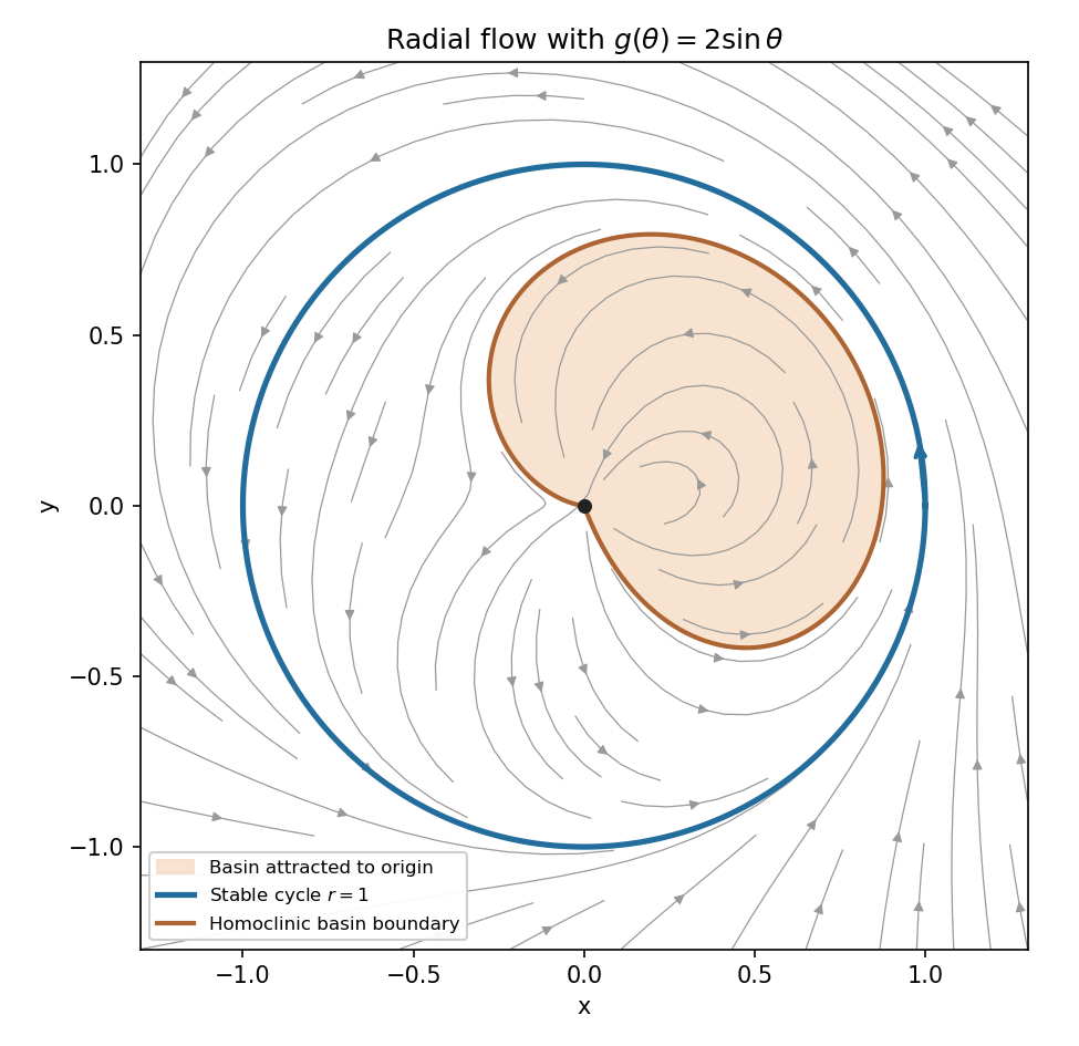
There are no other nonconstant periodic orbits: an orbit reaching the section with has strictly increasing successive values, and the remaining inner trajectories tend to the origin. The origin, defined by the continuous Cartesian extension, attracts the interior of the loop but is not Lyapunov stable, since arbitrarily small lower-sector initial points outside the loop approach the unit circle. This is the homoclinic basin boundary in a sinusoidal radial flow.
The two Gamma function integrals are absolutely convergent when . Consequently Fubini theorem givesMake the change of variables , , so , , , , and the Jacobian is . Powers of positive real variables use the real logarithm, so this transformation is also valid for complex exponents. The integral factors asBoth factors converge under the same real-part assumptions. The first is , proving the Beta function identity
Use the canonical Poisson bracket convention . The Hamiltonian flow generated by has and . The chain rule therefore givesThus is invariant under every such trajectory exactly when identically. Antisymmetry then gives along the flow of , so is a constant of motion.
For , the generated equations are , , hence , . Invariance under this simultaneous translation implies conservation of when ; the zero generator alone conveys no additional conservation law.
Write with and . The angular momentum component has and . Thereforesince a symmetric product contracts to zero with the antisymmetric Levi-Civita symbol. All three components of angular momentum are conserved by this rotationally invariant Hamiltonian.
Take velocities relative to a comoving observer at . Spatial homogeneity means that changing the observer to gives the same relative velocity law, soWith as origin this implies and . A physical velocity field is continuous; additivity first gives rational homogeneity and then, by continuity, real homogeneity. Hencewith coefficients independent of position. Without a regularity assumption, the additive functional equation alone admits non-linear pathological solutions; continuity is the usual implicit velocity-field assumption.
Isotropy requires for every spatial rotation, or . Rotations about force to be parallel to , and rotations exchanging coordinate directions force those diagonal coefficients to agree. Therefore and , the Hubble law.
The physical particle horizon is the greatest physical distance at time from which a light signal could have reached the observer since the beginning of the cosmological model. If that beginning is , radial null propagation has comoving distance , soFor and , the integral converges at zero and equals . ConsequentlyThe horizon problem is that widely separated regions of the observed cosmic microwave background have nearly equal temperatures although their past causal regions did not overlap before recombination in the usual decelerating hot-big-bang history. That history offers no causal equilibration mechanism for their observed uniformity. The particle horizon used here is distinct from the Hubble radius .
Define the Möbius function by , for a product of distinct primes, and if a prime square divides . For , summing over square-free divisors gives , while the sum is one at .
Both Dirichlet series and converge absolutely for . Their product may therefore be regrouped by the product of the indices:This simultaneously proves andIn particular .
Under the assumed analytic continuation, is holomorphic near when , and as . If were a zero of order , local factorization would give for sufficiently small positive . The preceding absolutely convergent bound gives instead , a contradiction. Thus . This reciprocal Dirichlet-series bound on boundary-zero multiplicity does not assert that any such boundary zero exists.
A model of three-dimensional hyperbolic space is with metric , the complete simply connected metric of curvature . The translation length of an isometry is . A hyperbolic isometry has positive translation length attained on its invariant complete geodesic, the axis of a hyperbolic-space isometry. It joins the two fixed ideal points and is translated by distance ; a three-dimensional axial isometry can also rotate around it.
For the boundary map , the hyperbolic extension of a Möbius transformation is . Every path from to has length at least the absolute change of , namely , because the metric length dominates . On the vertical line a vertical segment attains that bound. HenceIf the vertical line is the axis. If the map is a rotation with zero translation length, including the identity when ; it is not a positive-length hyperbolic isometry.
Represent the Möbius transformation by , which has determinant one and trace eight. Its distinct eigenvalues are and their product is one. A change of basis to eigenvectors conjugates its projective action to a dilation by or its reciprocal. Translation length is invariant under conjugacy, so part (i)'s dilation calculation givesThe fixed boundary points solve , namely . The axis of a hyperbolic-space isometry is the semicircular geodesic with those endpoints in the vertical real plane.
Put , which is positive definite because has full column rank. The log likelihood differs from by a term independent of . Differentiation gives the normal equations , henceThe distribution follows by writing and applying the linear transformation rule for a multivariate normal distribution.
Let and . Orthogonality of the residual to the columns of gives the exact decompositionThe prior is density proportional to with respect to . Thus the joint posterior distribution isCompleting the quadratic identifiesThe sampling distribution treats the true as fixed and varies the data, whereas the conditional posterior fixes the observed data and distributes . Their covariance formulas agree, but their centres and their interpretations differ.
For a new row vector , let and suppose its new error is independent. With known , the maximum-likelihood plug-in prediction uses mean and noise variance , while a calibrated frequentist prediction must account for the estimator: . If variance is estimated, the maximum-likelihood estimator is , whereas the exact frequentist prediction pivot uses and has Student t-distribution with degrees of freedom.
In the Bayesian calculation, integrating first gives . Integrating out of the joint posterior gives . For , integration of the predictive normal against this inverse-gamma distribution has density proportional toThe substitution reduces the integral to a Gamma function. Normalizing identifies the Student t-distribution, givingwhere the second parameter is a scale, not its variance. These Bayesian intervals coincide with the usual exact Gaussian-regression prediction intervals for this prior, although their probability interpretations differ. Posterior propriety requires and ; the former holds almost surely under the nondegenerate Gaussian model. Prediction of the noiseless conditional mean omits the added one in .
An interval covering relation means . The associated directed graph has one vertex for each interval and an edge for each covering. Its transition matrix is when that edge exists, and zero otherwise. Matrix multiplication counts walks; thus counts closed length- itineraries, with a distinguished starting vertex.
To see how itineraries force periodic orbits, a continuous map covering a closed interval has a closed subinterval mapping onto it: choose successive first/last crossings of its endpoints. Pull these subintervals back along a closed walk. This yields with . At the two preimages of the ends of , has opposite weak signs; the intermediate value theorem gives a fixed point of .
A graph alone does not give an exact count of periodic points for a general continuous map: extra oscillations or a fixed interval can create additional points. For example on , both and have matrix ; the first has infinitely many fixed points and the second only one. Distinct itineraries give distinct points when their interval interiors are disjoint and the periodic orbit avoids shared endpoints. In that setting, is a guaranteed lower bound, not a universal equality. Likewise, the primitive-word count counts guaranteed least-period itineraries under this separation condition. With overlapping intervals, even distinctness needs qualification. This is the scope of counting cycles in an interval covering graph.
For the first five-cycle, put , . The graph and matrix areThe four traces are . Shared endpoints have least period five, so they do not spoil the distinctness argument for the requested periods. Primitive cyclic itineraries are: for period one; for period two; and for period three; , and for period four. Consequently the monotone five-cycle interval covering pattern guaranteesThese words specify the successive intervals containing their points; cyclic rotations denote the same orbit.
There is a horseshoe for an interval map for : both and cover under that iterate, and their interiors are disjoint. Repeated binary choices produce at least separated length- itineraries for the second iterate, hence positive topological entropy, at least for . Thus the dynamics are chaotic in this standard interval-map sense. No conclusion of global transitivity on all of follows.
A one-step horseshoe is not guaranteed if that is the intended definition. For example the unimodal continuous map for and for has cycle . A left-branch interval cannot cover itself, since its image is shifted to the right. Two right-branch intervals cannot each cover their union because that branch is injective. If one interval straddles the maximum and covers itself, its right endpoint must map below its left endpoint; every disjoint interval farther to the right then maps below it and cannot self-cover. A disjoint interval to the left also cannot self-cover. So this example has no one-step two-branch horseshoe, although its second iterate does. It also proves that can be unimodal.
For the second order, write , , , . Endpoint images giveThe traces are . The guaranteed primitive words are , and , giving . To prove the last qualification, take ordered points and linearly interpolate the map values on , extending by for and for . Both exterior regions enter after at most two steps, so they introduce no extra periodic points. Its only closed length-three itinerary is ; on it is , whose third iterate has only the same fixed point. Endpoints have least period five, so this example has no three-cycle.
The distinct fourth-iterate return walks and yield two subintervals of that return over , giving a horseshoe for and positive entropy at least . Thus too must have chaotic interval dynamics and a horseshoe in some iterate. The affine example has no one-step horseshoe: its increasing branch lies strictly below the diagonal, while on the decreasing branch injectivity prevents two self-covering intervals; a minimum-straddling self-covering interval excludes a self-covering interval on either side by the same endpoint argument. The distinction between a map and its iterate is essential for both patterns.
Put . The Hamilton equations areDifferentiate the mechanical momentum and substitute:With and in this zero-scalar-potential gauge, this is , the Lorentz force in the units of the Hamiltonian.
For , is cyclic, so is conserved. Choose , giving , where . Since , its Hamilton equation gives , henceFor nonzero constant , the orbit is an ellipse of semiaxes and . Its enclosed phase-space area is , so the action variable isThe absolute value keeps the action positive if the signed charge or magnetic field is negative.
When the field varies slowly along the trajectory, with and no zero-frequency crossing, adiabatic invariance of the action makes approximately constant. Thus and the slow motion has effective HamiltonianThe effective potential is the second term. Direct averaging checks its force: the exact equation is , while the oscillator has . Hence . Spatial field variation along the slow motion must satisfy the same adiabatic condition; slow explicit time variation alone does not control passage through a sharp spatial gradient. A time-dependent effective potential need not conserve total energy.
A transitive class satisfies . Its membership structure therefore does not omit elements of its members. In particular bounded membership statements are absolute between a transitive model and the ambient universe, and its membership relation is the actual well-founded relation, rather than an arbitrary externally ill-founded coding.
For a set , put and , and defineThis is a set, contains as a subset, and is transitive: an element of an element of belongs to . Any transitive set containing as a subset contains every by induction, so this construction is the least such set. Shifting the union index givesThese formulas use the specified subset convention for transitive closure.
Work in the usual ambient set theory with Choice. If is a hereditarily countable set, then every member of is countable. Iterated countable unions show that this entire closure is countable. Conversely a countable transitive closure makes each of its members countable. This equivalent criterion makes the following closure arguments explicit.
If , then , so : HC is transitive. If , its union is countable and its descendant sets are descendants of , so . The actual union therefore witnesses the Axiom of union inside .
For axiom schema of separation, take any formula with parameters in HC and a set . Form the subset of consisting of the elements that satisfy that formula with all quantifiers relativized to HC. Ambient Separation supplies this set. It is a subset of a countable set, and all its descendants are inherited from , so it belongs to HC. No claim that the formula itself is absolute is needed.
The axioms satisfied by hereditarily countable sets also include Extensionality, Empty Set, Pairing, Infinity, Foundation and Replacement. Extensionality and Foundation follow from transitivity and ambient well-foundedness. Empty Set and belong to HC, and a pair of HC sets has countable transitive closure. For Replacement, the domain is countable; a definable image of its elements is a countable family of HC sets, whose combined transitive closures form a countable union of countable sets, so the range again belongs to HC. Ambient Choice additionally gives Choice internally: a well-order of a countable HC set has a hereditarily countable relation and hence lies in HC.
Power Set fails. Every subset of is hereditarily countable, so an internal power-set witness would have to contain all ambient subsets of . That collection is uncountable by Cantor theorem, whereas every HC set is countable. Thus HC satisfies the other ZF axioms and, in this ambient setting, Choice, but not the Axiom of power set.
For each vertex triple , let indicate that its three edges are present. Then andEach variance is . Two distinct triples have independent indicators unless they share an edge; in that case their covariance is . There are unordered pairs sharing an edge. Therefore the triangle count in a binomial random graph hasIf , Markov inequality gives . If , then andThe second term tends to zero since . Chebyshev inequality now gives , proving the stated threshold. Here the random-graph phrase “almost surely” means asymptotically almost surely, that is, with probability tending to one.
At , let count edges. Direct subtraction givesSome graph has at least this expectation. Successively deleting one edge from each remaining triangle destroys all triangles with at most deletions, so a triangle-free graph remains with at least edges. This triangle deletion in the alteration method proves the requested existence bound.
It is not within a constant factor of the optimum. A balanced complete bipartite graph has edges and no triangle. Conversely, in a triangle-free graph each edge satisfies . Summing over edges gives , where is its edge count. Cauchy-Schwarz inequality gives , hence . The optimum is therefore , quadratic rather than the obtained bound.
A primitive root of unity satisfies and for , equivalently it has multiplicative order . A positive characteristic of a field must be prime: if its least positive value factored as with , the two nonzero field elements and would have product zero. If this prime divides , put . In characteristic , the binomial coefficients for vanish because their integer numerators contain and their denominators do not. Thus . It follows that . A field has no nonzero nilpotent element, so , contradicting primitivity. Consequently .
A primitive tenth root has and , so division of by givesIt is irreducible over : replacing by gives , and then replacing by gives . Any nontrivial monic integer factorization would reduce modulo five to factors that are powers of , forcing both constant terms divisible by five and their product divisible by , contrary to the constant term five. Rational factorization reduces to integer factorization by Gauss lemma: products of primitive integer polynomials are primitive, since reduction modulo any prime preserves a nonzero product. ThusLet . Dividing by gives . Hence , so . Either sign of this square root suffices; for the positive one is .
A finite field contains a primitive tenth root exactly when . Its multiplicative group is cyclic: the exponent of a finite abelian subgroup of a field is attained by an element, by combining its prime-power components; since every element is a root of , the polynomial root bound forces the group order to be at most that exponent, hence equal to it. A cyclic group contains an element of order ten exactly when ten divides its order.
Over , the conjugates of are its Frobenius automorphism orbit . The extension degree is the least with . For this order is four, for it is one, and for it is two. Therefore
The restriction of a representation to is the same vector space and operators with the domain limited to ; its character is . Averaging a positive Hermitian inner product over makes it invariant, so invariant subspaces have invariant orthogonal complements. Repeating gives a direct sum of irreducible -spaces and hence with nonnegative integer multiplicities.
By character inner product orthogonality,since is irreducible and has normalized squared norm one on . Equality holds precisely when the omitted nonnegative terms vanish, namely . This is the restriction multiplicity bound.
The induced character construction extends any class function on byFrobenius reciprocity for class functions is . It follows directly by substituting this sum into the left inner product, writing , and using the conjugacy invariance of . If is a character, its inner product with every restricted irreducible character is a nonnegative integer, a multiplicity in its complete reducible decomposition. Expanding in the orthonormal irreducible-character basis therefore makes a nonnegative integer sum of irreducible characters: it is a character of .
If affords , a concrete induced representation is , with acting by left multiplication on the first factor. Choosing coset representatives decomposes it into copies of . An element permutes these copies; only fixed cosets contribute trace, and the contribution from is . Summing fixed cosets gives exactly the displayed induced class function.
Let , extend to by zero outside , and choose coset representatives . Then with . Each summand has squared -normsince is irreducible. Pointwise Cauchy-Schwarz inequality gives . After summing and dividing by ,The are nonnegative integers by part (b). This proves the character induction norm bound without an assumption that is normal.
Choose the real embeddings and one from each complex pair . The logarithmic embedding of number field units isIt is a group homomorphism from multiplication to addition. A unit has absolute norm one, so the coordinate sum is zero and its image lies in a Euclidean hyperplane of dimension .
Here is the required discreteness argument. There are only finitely many algebraic integers of whose conjugate absolute values are bounded by a fixed constant: their monic minimal polynomials have degree at most , and each integer coefficient is an elementary symmetric function of bounded roots, hence belongs to a fixed finite range. There are finitely many such polynomials and finitely many roots of each. A bounded set of logarithms bounds all conjugate absolute values, so every compact region in the logarithmic hyperplane meets the unit image in finitely many points. Thus the image is a discrete additive subgroup.
Use the allowed Euclidean-group theorem: a discrete subgroup of a finite-dimensional real vector space is free abelian on finitely many vectors, with rank at most the dimension. Therefore has rank at most . Its kernel is finite by the same bounded-conjugate argument, now with every absolute value one. Each element of a finite multiplicative group is a root of unity, and conversely every root of unity has all logarithms zero. Thus the kernel is exactly the finite group of roots of unity, and exactly the torsion subgroup of units.
Lift generators of the free logarithmic image to units; together with the finite kernel they generate every unit. HenceThis proves the requested upper bound without invoking the existence half of the Dirichlet unit theorem. The field is a subfield of , and its only real roots of unity are .
Use integral homology groups. The sphere is ; each disk meets in its boundary circle, while . In particular, the two disks also meet away from the sphere. These spaces have compatible triangulations, so the Mayer–Vietoris sequence applies to their unions as subcomplexes; equivalently use small regular open neighborhoods with the same homotopy types.
First let . Its intersection is , and is contractible. The Mayer–Vietoris sequence givesFor example, the degree-two portion is , and the map from into is injective.
Now . It has and . Exactness gives andThis sequence splits: lift a generator of the quotient and extend its lift by integer multiples. Hence . In degree one the sequence becomesThe middle map has kernel generated by and cokernel . There are no higher groups, either by the same sequence or by the three-dimensional triangulation. Thus the homology of two disks meeting inside a sphere givesThe first-homology generator records a path from the sphere to the common interior point through one disk and back through the other; omitting that interior intersection would incorrectly remove this generator.
For a complex Banach space, the spectrum of a bounded operator and resolvent set areThe bounded inverse theorem says that a bounded bijection between Banach spaces automatically has a bounded inverse, so failure of bijectivity suffices here. The point spectrum isthe set of eigenvalues. For a real Banach space, these definitions use its complexification.
A compact operator is a bounded linear operator carrying every bounded set into a relatively compact set. Equivalently, for every bounded sequence , the sequence has a norm-convergent subsequence. It is enough to require this for the closed unit ball, because any bounded set lies in a scalar multiple of that ball.
Suppose otherwise and choose linearly independent eigenvectors with and . Put . Each is finite-dimensional and -invariant. Moreover , including when some eigenvalues coincide.
Apply the supplied distance fact inside the Banach space to choose with and . For , both and belong to . ConsequentlyThus has no Cauchy subsequence, although is bounded. This contradicts the compact operator property. Only finitely many linearly independent eigenvectors can have eigenvalue modulus greater than .
The exact condition for this diagonal operator on sequence space isFirst, is bounded precisely when , with operator norm equal to that supremum: the upper bound follows by summing , and the coordinate unit vectors give the lower bound. If the supremum is infinite, choose distinct indices with and set , other coordinates zero. Then but , so the displayed prescription would not even define an everywhere-defined map into .
If is compact but , infinitely many indices satisfy . Along those indices,contradicting compactness. Conversely, if , truncate to . This is a finite-rank compact operator, and . To see compactness directly, approximate the image of the unit ball by to within , and cover its bounded finite-dimensional image by finitely many -balls. Hence 's unit-ball image is totally bounded; its closure is compact because is complete.
For a smooth projective curve of genus , the Riemann-Roch theorem stateswhere is a divisor, a canonical divisor, and . In particular, applying it to and gives and .
For a nonconstant morphism of degree in characteristic zero, choose local parameters with up to a unit at a point of ramification index . Pulling back a differential multiplies its local order by and adds , because and in the field. ThusThe degree of a divisor of a pulled-back divisor is times its degree. Taking degrees and using the Riemann-Roch theorem gives the Riemann-Hurwitz formula
A smooth plane cubic has genus one by the genus-degree formula. In the displayed normal form, with : otherwise divides and the cubic is reducible. Therefore the line meets the cubic in the divisor , and . The elliptic curve group law identifies with the degree-zero divisor class . Order three means . Consequently and has a section with zero divisor .
Every section of is the restriction of a linear form: ambient linear forms form a three-dimensional space and restrict injectively, while Riemann-Roch theorem gives , since forces the dual term to vanish. Thus this section is some nonzero , proving , with intersection multiplicity three. This is the three-torsion points are flexes of a plane cubic property.
Projection forgetting defines a morphism : its only possible indeterminacy point does not satisfy the second equation. It is a double cover. Away from the zeros of , its two square roots are distinct. Each line intersects in three simple points, since it is nowhere tangent; the two triples are disjoint because the lines do not meet on . In a local trivialization near any of these six points the covering equation is with , so the ramification index is two. There is no other ramification. The Riemann-Hurwitz formula therefore gives
The global Gauss-Bonnet theorem for the induced Riemannian metric isHere is the Gaussian curvature, the induced surface-area element, and the Euler characteristic. For a connected orientable compact surface of genus , . For several components, sum their contributions. There is no boundary-curvature term because has no boundary.
A parametrized curve is a geodesic when its covariant acceleration vanishes, , for the induced Levi-Civita connection. In coordinates this isEquivalently, for an embedded surface its ordinary acceleration is normal to the tangent plane. The parameter is affine; arbitrary reparametrizations need not remain geodesics.
The local existence and uniqueness theorem says that for every and there is a unique geodesic with , , on a maximal open interval containing zero, depending smoothly on . This follows from the local existence and uniqueness theorem for the smooth first-order system in . The exponential map is wherever the solution exists through time one. Its domain contains a neighborhood of zero, and , since . Thus it is a local diffeomorphism near zero. Completeness is not assumed for a general surface; on a complete surface it is defined on all of .
An isometry preserves the Levi-Civita connection. To justify this, transport the connection on by . It is torsion-free and preserves the metric on , since preserves the metric and Lie brackets. These two properties characterize the Levi-Civita connection uniquely: if two such connections differ by , the tensor is symmetric in its first two arguments and antisymmetric in its last two. Cycling these symmetries yields , hence . ThereforeApplying this along shows that the covariant acceleration of is zero, so an isometry carries affinely parametrized geodesics to geodesics.
The same identity and the definition show that intertwines the Riemann curvature tensor. If is an orthonormal tangent basis, its image is orthonormal and
Both proposed converses are false. Take with the Euclidean metric and . A geodesic maps to the geodesic , and both Gaussian curvatures vanish identically. Nevertheless multiplies lengths by two, so is not an isometry. This one counterexample answers both unheaded continuation requests.
Let be the linear subspace of consisting of classes admitting -measurable representatives. It is closed. Indeed, if converges in to , choose a subsequence converging almost surely: take and apply Markov inequality and the Borel-Cantelli lemma to errors exceeding . The pointwise limit of its -measurable representatives, set to zero wherever the finite limit does not exist, is -measurable and equals almost surely. This also works when is not complete.
Here is a proof of the orthogonal projection construction using only completeness. Put and take approaching this infimum. The parallelogram law givesCompleteness and closedness give a minimizer . For every , expand for real . Its minimum at zero impliesThis is unique almost surely, because the difference of two possible choices belongs to and is orthogonal to itself. It is the conditional expectation , as also follows by testing indicators of events in .
For the jointly Gaussian pair, if , setThe residual has mean zero and covariance . Since is jointly Gaussian, its characteristic function factors when this covariance is zero, so and are independent. Hence for every square-integrable function of ; independence first proves this for bounded functions, and truncation plus Cauchy-Schwarz inequality gives the general case. This proves the Gaussian conditional expectation formula, including a zero residual variance. If , almost surely and the covariance inequality gives ; is the answer.
Number the vertices by . The continuous-time Markov chain moves one step forward cyclically at rate one, as shown in the left diagram.
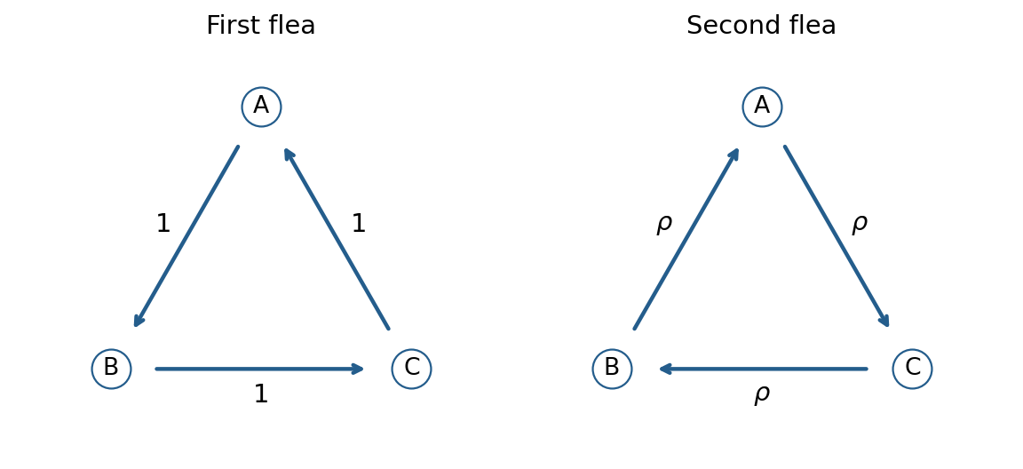


Write for the cyclic shift matrix, so . With , the eigenvalues of are and those of areThe stationary distribution is uniform. A jump count is a rate-one Poisson process, and the displacement is that count modulo three. The roots-of-unity filter and therefore give, for ,These are also the entries of obtained by diagonalizing . In particular,
The second continuous-time Markov chain runs in the reverse direction at rate , as in the right diagram. Its nonzero eigenvalues have real part , and its transition probabilities tend to for each vertex. Independence therefore givesThus the limit exists for every pair of starting vertices and equals .
One can also see the limit directly without spectral multiplication. For fixed starting vertices, modulo three advances with each jump of either flea. Its jump count is the sum of independent Poisson processes with rates and , hence is Poisson with rate (multiply their generating functions). The formula from part (a), with replaced by and the appropriate initial residue, gives and the same limit.
Write for the two simple hypotheses, with prior probabilities and densities . Under zero-one loss, the posterior expected losses of choosing and are respectively the posterior probabilities of and . A Bayes decision rule therefore chooses ifchooses for the reverse inequality, and may randomize at equality. With positive priors this is a likelihood-ratio test with cutoff .
For a test , its prior risk is . Choose and boundary randomization so that the likelihood-ratio test has size , and choose priors with ratio . Equivalence of normal and extensive analyses makes the pointwise posterior minimizer minimize this prior risk over all randomized tests. Thus for any ,This proves the Neyman-Pearson lemma: a likelihood-ratio test of size has greatest power among tests of size at most . Such a cutoff and randomization come from a quantile of the likelihood ratio under ; always reject where . Endpoint cutoffs are handled directly or by their limiting rules.
For the remaining assertions use the usual common-support formulation with positive densities. A family has a monotone likelihood ratio in if for every , is a nondecreasing function . A monotone test here is an upper-cutoff test , , including constant tests. It does not mean an arbitrary smoothly increasing randomized rejection function.
Put . For a finite cutoff, choose between the values of below and above , with when the boundary has positive probability. On , and ; on , both are nonpositive. At a boundary with positive mass . ThereforeWhen there is probability on both sides, finite positive monotone ratios below the cutoff bound those above it away from zero, so can be positive and finite. A boundary with positive mass instead supplies the positive finite value . If the cutoff yields a constant test on the support, positivity on the common support proves strict propagation directly: a test identically zero cannot have greater power, and for a test identically one any positive-probability nonrejection by the competitor remains positive-probability at the larger parameter. Hence implies .
Let , taking when this set is empty. Below there is no positive difference. Above a finite there is a smaller parameter with positive difference, which propagates upward; the same reasoning applies when . ThusNo assertion at itself is needed.
For the final request fix any cutoff and prior density . Set and . The posterior odds are . If , thenEvery bracket is nonnegative by monotone likelihood ratio. Equal statistics make the bracket zero, so the ratio depends only on . Dividing where the posterior is defined proves the posterior odds are nondecreasing in , with extended values allowed when one posterior mass is zero. This proves that posterior odds are monotone under a monotone likelihood ratio without restricting the prior's shape.
The common positive-support condition is material to the printed strict inequality. Under the broader definition permitting zero densities, take a two-parameter family on with and . Its likelihood ratio is nondecreasing. The cutoff test rejecting has greater power than the test rejecting only at parameter zero, but both have power one at parameter one. Thus the strict assertion needs the usual positivity convention; it is false without it.
Pontryagin maximum principle leaves the initial costate unknown. Terminal conditions determine these unknown constants and, when terminal time is free, the time. In a maximization convention with terminal reward and running cost , use . A free terminal coordinate gives ; a fixed terminal coordinate instead allows a constraint multiplier. More generally is normal to the permitted terminal manifold. The free-terminal-time transversality condition is . These conditions convert the adjoint and state equations into a boundary-value problem. Reversing the costate sign gives the equivalent minimization convention.
Maximize . Along the positive- trajectory use Hamiltonian of an optimal-control problem . The terminal costate is , andThus . Maximizing over gives as long as . The state equation integrates to , and the adjoint equation gives , validating the maximization. HenceThis is globally optimal, not just an extremal: whenever , . If a competitor reaches and later becomes positive, apply that bound after its last zero; it has even less remaining time to attain a positive terminal height. A negative terminal height cannot improve this positive maximum. Therefore the minimum objective is .
Articles were limited to the first 100 out of 134 total.
Articles by others on the same topic
There are currently no matching articles.