Linearity of the integral in each argument gives a bilinear form, and gives symmetry. Also . If a polynomial is nonzero somewhere on this interval, continuity makes strictly positive on a smaller interval, so the integral is positive. A polynomial vanishing on the whole interval is the zero polynomial. Thus the form is positive-definite and is an inner product.
Apply the Gram-Schmidt process to . Odd functions have zero integral, so is already orthogonal to , and the third orthogonal polynomial is . Their squared norms areTherefore an orthonormal basis isThese are the first three normalized Legendre polynomials. Their distinct degrees also prove that they span the three-dimensional vector space.
The group presentation gives the quotient group by the subgroup generated by the rows ofFor the Smith normal form, the first determinantal divisor is the greatest common divisor of all entries, namely . The nonzero two-by-two matrix minors are , so the second determinantal divisor is . The third row is the second minus the first, and a nonzero minor shows the rank is exactly two. Consequently the nonzero invariant factors are and , with one free generator. The Fundamental theorem of finitely generated abelian groups givesAn element killed by has zero free coordinate, arbitrary coordinate in , and coordinate or in . There are nine such elements. Removing the identity leaves eight elements of order three.
A contraction mapping on a metric space satisfies for all , with one constant . The contraction mapping theorem says that on a nonempty complete metric space such a map has a unique fixed point; successive iterates from any starting point converge to it. More precisely, if , then .
The Volterra integration operator maps continuous functions to continuous functions. In the uniform norm,This constant cannot be decreased: for and , , and both uniform norms are one. Hence is not a contraction.
Changing the order of integration over the triangular region givesThus is a contraction, with sharp constant . This is an example of an iterated contraction.
For an entire function, the Cauchy derivative formula on a positively oriented circle of radius about isThe resulting Cauchy estimate is , where is the maximum of on that circle.
The Liouville theorem says that a bounded entire function is constant. Indeed, if on the plane, the Cauchy estimate with gives . Sending to infinity gives at every point, hence is constant.
For the growth assumption, apply the Cauchy estimate on circles centred at zero. For every integer ,All sufficiently high Taylor series vanish. Since the Taylor series of an entire function converges everywhere, is a polynomial, of degree at most when . If a negative finite exponent is interpreted for nonzero , the same estimate forces every coefficient to vanish, giving .
Away from zero the Dirac delta distribution is absent. On either half-line, use and the power-law ansatz . The Euler-Cauchy equation becomesThe growing term is excluded by boundedness at either end. Thus the independently bounded half-line solutions are
The sign of the Dirac delta distribution in the equation is positive after the outer minus sign is expanded. Integrating through zero, the nonsingular potential contributes a term tending to zero, whereas the delta term contributes . The jump condition for an impulse is thereforeContinuity at zero gives . The two one-sided derivatives are and , whose difference is exactly . Hence the matching condition introduces no further restriction on , and the globally bounded solution isThis continuous solution has precisely the derivative jump required for its second distributional derivative to cancel the delta term. Its amplitude remains arbitrary because no normalization has been imposed.
For a normalized state and a self-adjoint operator with finite second moment, the quantum uncertainty is defined by . Since is real,In an energy eigenstate of the quantum harmonic oscillator,Discarding the nonnegative squared means proves the stated lower bound. The Heisenberg uncertainty principle is , following from . Applying the arithmetic-geometric mean inequality to the two variance contributions givesHere is the oscillator frequency. The bound is the ground-state energy; equality requires zero means and the appropriate minimum-uncertainty width.
Use the ideal long-solenoid approximation: negligible pitch and end effects, vacuum permeability , and negligible displacement current. By cylindrical symmetry the magnetic field is axial. An Ampère's law rectangular loop with one axial side inside and the other outside gives . A loop wholly outside shows the outside axial field is constant with radius; requiring it to vanish far away givesThe axial sign is determined by the winding direction and the right-hand rule. The small axial component of current from the spiral pitch is neglected in this idealization.
There are turns, and the magnetic flux through each is . The flux linkage is , so the self-inductance isThe induced electromotive force opposes increasing current by Faraday's law. Together with Ohm's law, the circuit equation is . Solving this first-order ordinary differential equation with givesThe time constant is , and the limiting current is .
For any distinct nodes, the polynomial has degree , is nonnegative, and vanishes at every node. The quadrature rule sum for is zero, but because the weight is positive and is positive except at finitely many points. Therefore no such rule is exact for all polynomials of degree at most , irrespective of the chosen weights.
For the sine weight, its first four moments are . A monic degree-two orthogonal polynomial issince direct use of these moments gives . Its roots lie in and areThe weights follow by requiring exactness for and : and , and the symmetric nodes imply both weights are one. To prove cubic exactness, divide any cubic as , with of degree at most one. The integral of is zero by orthogonality, and its nodal values vanish; the remaining linear polynomial is integrated exactly. This is the two-node Gaussian quadrature with sine weight; the argument proves its Gaussian quadrature property without assuming a general quadrature theorem.
The Markov property and the Chapman-Kolmogorov equation giveFor each intermediate state, one first uses the next-step transition probability and then the following one; the sampled history adds no information once is known. Thus is a homogeneous Markov chain with transition matrix and initial law . In particular,If zero is not a state of , this probability is zero.
The authoritative definition here is . On the conditioning event, . Since , the additional condition then forces . The Markov property therefore givesAs usual, this conditional probability is asserted when the conditioning event has positive probability.
Starting from forces . The first nonzero value is consequently . Remaining nonzero at the next step forces , because . Hence, on an event of positive probability,The two values are unequal by assumption. They expose memory of the hidden sign: immediately after leaving zero the sign is negative, whereas after two consecutive nonzero observations it is positive. Whenever the relevant observed histories coexist with positive probability, the Markov property for fails, since its next-step law is not determined by its present value alone. In particular, the absolute-value projection does not preserve the Markov property for all initial laws; the strong lumpability condition would require .
There is a small qualification to a blanket conclusion about an unspecified initial law. The printed assumptions do not ensure that either conditioning event is possible, and a degenerate initial law may never reach the hidden states that cause the failure. For example, in the order , takeAll printed constraints hold, yet always and is a Markov chain. Thus the correct general conclusion is the transformed process is not necessarily Markov; the two computed probabilities give the intended failure when their histories are available.
The algebraic dual space is , the vector space of all real linear functionals. For a finite basis , define the dual basis by , so . Every linear functional satisfiesThis equality follows by evaluating both sides on each vector of the basis. It proves spanning directly. If , evaluation on gives , proving linear independence without assuming a theorem on dual dimensions.
For a vector subspace , its annihilator of a vector subspace isExtend a basis of to a basis of . Then has basis , so .
The dual map of is , . In the corresponding dual bases its matrix is the transpose of the matrix for . A matrix and its transpose have the same rank, giving . Directly,Thus . Also every vanishes on , so . Both spaces have dimension by the preceding annihilator of a vector subspace formula and rank-nullity theorem, provingAlternatively, a linear functional vanishing on the kernel descends to the image of and can be extended to by extending a basis.
For the infinite-dimensional polynomial ring, the coefficient functionals are linearly independent: evaluate a finite relation on each monomial. However, they do not span the algebraic dual space. The linear functional takes value one on every monomial, while any finite combination of the vanishes on every sufficiently high-degree monomial. Thus the do not form a basis of . An infinite formal sum of coefficient functionals is not a finite linear combination.
With the usual commutative, unital conventions, the chain isA field is an integral domain, and every nonzero ideal contains an invertible element and is consequently the whole ring. Its only ideals are and , so it is a principal ideal domain.
To prove the middle implication, first show that a principal ideal domain has the ascending chain condition on ideals. The union of an ascending chain is an ideal, hence is ; its generator belongs to one member of the chain, and all later members equal . Now suppose a nonzero nonunit admitted no factorization into irreducible elements. It would factor into two nonunits, at least one of which again has no such factorization. Repeating would produce a strictly increasing chain of principal ideals: if with a nonunit, , since equality and cancellation would make invertible. This contradicts the ascending chain condition. Existence of factorization follows. By the permitted fact that every irreducible element is a prime element in a principal ideal domain, any irreducible factor in one factorization divides a factor in the other; cancellation then proves uniqueness up to units and order. This is a unique factorization domain. The final implication is part of the definition of a unique factorization domain.
None of the adjacent implications reverses. The principal ideal domain is not a field, since is not invertible. The polynomial ring is a unique factorization domain, by applying the polynomial extension theorem for unique factorization domains twice, but its ideal is not principal: a generator would divide both and , so would be a unit, whereas every member of this ideal vanishes at the origin. Finally, is an integral domain as a subring of , but is not a unique factorization domain. Its multiplicative norm is . There is no element of norm or . Hence , of norms , are all irreducible: a nontrivial factorization would require one of those missing norms. The only units have norm one and are . The two factorizationsare therefore not related by associates and reordering.
The set is the ideal quotient . It contains zero. If , then , since is an subgroup. If and , then because is an ideal. Thus is an ideal.
Write and . Because , each has the form . Then , so , and . Conversely by the definition of . Thereforeso is a principal ideal. This argument uses only the commutative ring convention, not cancellation or an integral domain hypothesis.
To prove the sufficient condition, take a rectangle about contained in the open domain. Split the increment along its coordinate directions:The one-variable mean value theorem, applicable because the restrictions are differentiable, represents these two terms asThe zero-increment cases are interpreted directly. Subtract . By continuity of both partial derivatives at , the remainder is at most once the increment is small. This is the required little-oh remainder and proves differentiability.
The converse is false. Set for , and . At each point with , its Frechet derivative is zero, since the function increment has magnitude at most . It is smooth away from this line. Butis not continuous there. Thus a function can be differentiable everywhere while its partial derivatives are discontinuous.
For , every point with is a smooth point. At the origin, , so is differentiable with zero derivative. At with , the putative first partial derivative would require the limit , which does not exist. Consequently the exact set of differentiability is
A metric space is complete if every Cauchy sequence in it converges to a point of that space. The stated shrinking-set characterization is the Cantor intersection theorem together with its converse.
First assume completeness, and choose . If , then both points belong to , so . The vanishing diameters imply that is a Cauchy sequence, hence it converges to some . For every fixed , its tail belongs to the closed set , so . Thus . In fact the intersection contains only one point, since any two of its points have distance at most every diameter.
Conversely assume the stated intersection property and let be a Cauchy sequence. PutThese closures are nonempty, closed and nested. Taking a closure does not increase the diameter: approximate two points of the closure by points of the set and use continuity of distance. The Cauchy sequence therefore makes . Choose in the intersection. For , both and belong to , and . Every Cauchy sequence converges in , proving completeness.
Take the incomplete metric space with its usual distance, andEach is nonempty and closed relative to : it is . The sequence is strictly descending and its diameters are . Its intersection is empty, since every positive point exceeds for sufficiently large . The excluded limiting point is zero.
In , takeThese are nonempty descending sets of diameter , with empty intersection. They are not closed sets, so there is no contradiction with the Cantor intersection theorem for the complete metric space .
In , takeThe sets are nonempty, closed and strictly descending, but their intersection is empty. Their diameters are infinite, so the shrinking-diameter assumption is essential.
For , integration by parts recursively in the Laplace transform givesThe initial exponential boundary term vanishes, and starts the recursion. Here is the Heaviside step function.
Transform the displacement in time, writing . Zero initial displacement and velocity give . A particular solution is , and the spatial homogeneous solutions are . The prescribed far-field behavior excludes the growing exponential. The fixed boundary sets the remaining coefficient to , henceSince , the Laplace transform time-shift rule givesEquivalently, for , and for . This solves the forced wave equation in each region and has continuous displacement and first derivatives across the characteristic , so it also solves the equation weakly there. It satisfies the fixed-end and initial conditions and equals sufficiently far away at each fixed time. The end's influence travels at speed .
An embedded surface parametrization is a smooth map , with open , injective differential of rank two at each point, and a homeomorphism onto its image with the subspace topology. Its induced metric isIn coordinates, an arc-length-parametrized geodesic satisfieswhere the Christoffel symbols are . The normalization fixes unit speed; it is compatible with the differential equations because geodesic speed is constant.
For the cone use , , restricting to a suitable open interval for a chart. Direct differentiation gives its first fundamental formWith and , this becomes , the Euclidean metric in polar coordinates. The map is therefore a local isometry. It is local rather than global because increasing by increases by .
Given two points, choose their angle representatives so that . Their developed plane angles then differ by at most . The straight segment between their developed positions stays away from the origin: it lies in an angular sector of width at most containing both positive-radius endpoints. Develop that segment back onto the cone. Since local isometries preserve geodesics, it gives a geodesic joining the two points; it can be parametrized by arc length. This constructs geodesics on a punctured circular cone. For a repeated point the constant curve is the degenerate geodesic. In particular, this argument does not appeal to completeness of the punctured cone.
The joining geodesic need not be unique. For endpoints with equal positive radius and opposite azimuth, one may use the angular changes and . In the plane these give two straight segments from to and , respectively. Both avoid the origin. Their lifts pass on opposite sides of the cone and have distinct images, so a reparametrization cannot identify them.
Along a sufficiently smooth stationary curve, differentiation and the Euler-Lagrange equation give the Beltrami identity:The cancellation uses the absence of explicit dependence.
For an axisymmetric surface of revolution, its area is . A smooth positive-radius minimizer is stationary, so the Beltrami identity, with the constant factor omitted, givesEquivalently the Euler-Lagrange equation gives , whence . The first integral selectsEqual radii at imply (subtract the two cosh values), givingThis is a catenoid. The conclusion is a necessary form for a smooth connected minimizer; it does not declare every stationary catenoid a minimum.
Put . The boundary equation is . Its derivative is , so its unique critical point solves . The left side increases strictly from zero to infinity. Thus decreases to a unique minimum and then increases, diverging as and . There are exactly two positive values of whenAt equality there is one value, and below it there is none.
To match the printed second variation convention, write ; its is the quadratic coefficient, half the second derivative with respect to . Expanding the area integrand givesOn the catenoid these coefficients are and . Integrate the mixed term by parts; the boundary term is zero because . Since , this yieldsThis is the axisymmetric second variation of a catenoid, with the explicitly stated quadratic-coefficient convention.
The complex Fourier series of a -periodic function isThe coefficient formula follows from orthogonality of the exponential functions. For an arbitrary square-integrable function, this representation means convergence in the norm. With appropriate additional regularity it also gives pointwise convergence, to the mean of the one-sided limits at a jump. No pointwise representation is asserted for an unrestricted function merely from periodicity.
The Parseval identity for a complex Fourier series isIt holds for every square-integrable function, with complex conjugation expressed by the absolute squares. It is the Pythagorean theorem extended to the complete orthonormal system of complex exponentials.
Integrate the two exponentials in against . For there are no zero denominators, andThus the complex Fourier series isThis is the periodic extension, not a globally nonperiodic cosine formula. For each fixed complex , the coefficients are , giving absolute and uniform convergence. The extension is continuous at the endpoints because the two endpoint values agree; piecewise smooth pointwise convergence of a piecewise smooth Fourier series identifies the sum with it, including those endpoints.
Evaluate the absolutely convergent complex Fourier series at . The factors equal one, and the term is . Pairing positive and negative integers givesSince for nonintegral complex , rearranging provesThe last term means , so half-integer arguments are included by the finite cotangent value zero.
For real nonintegral , the Parseval identity and the coefficient formula giveSolving for the sum yieldsAt , the sine square is one and the cotangent is zero, giving .
Apply mass conservation to a fixed horizontal region . The layer mass is and the outward horizontal flux is . The divergence theorem and arbitrary choice of giveThis depth-integrated law retains free-surface motion; neglecting the vertical velocity in horizontal momentum is not the assumption that the depth cannot change.
Take the free-surface pressure to be constant. hydrostatic pressure gives , so the horizontal pressure forces are . Linearization about a resting layer gives the linearized shallow water equationsTaking the curl of the momentum equations yields . Combining with continuity gives the linearized shallow-water potential-vorticity anomalyFor , . Taking the divergence of momentum gives . Eliminate the divergence with continuity to obtainFor , substitution of gives the inertia-gravity wave dispersion relationThe associated purely oscillatory velocity field isThese formulas satisfy all three linearized equations and the zero-anomaly condition. A separately added spatially uniform inertial oscillation is not part of this monochromatic wave.
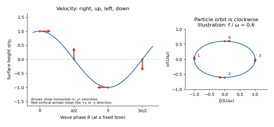
To first order in amplitude evaluate the wave at a particle's equilibrium coordinate , so . Integrating its velocity gives displacements relative to the orbit centreThese are particle ellipses for rotating shallow-water waves, with axis ratio . For the stipulated positive signs, the velocity at phases points respectively right, up, left, down, with magnitudes . The particle orbits are clockwise as time advances, since the phase decreases.
For the normal linear model, differentiating the ordinary least squares objective gives . Full column rank makes invertible, soThe distribution follows because is a linear transformation of a multivariate normal distribution. Its expectation is , and direct multiplication gives the displayed covariance matrix.
Let , the orthogonal projection onto the design's column space. The residual sum of squares is . Since , symmetry and idempotence give . Thusis an unbiased estimator.
For the two independent regressions choose . The first rows of the design matrix are and the last rows are . The centering conditions and distinct predictors giveIt follows thatThe two estimated slopes are independent normal random variables, as they depend on independent error blocks. ThereforeFor these data use the pooled residual sum of squaresIts scaled value is and is independent of the slope estimates by the permitted normal-model result. Hence the standardized difference has a Student t-distribution with degrees of freedom, giving the exact 95 percent confidence intervalHere is the 0.975 quantile of that distribution. This is a confidence interval for the difference of independent regression slopes. As required by the original framework, this specialization needs . Distinct predictors alone allow , but then the fit is saturated, and there are no residual degrees of freedom to estimate the unknown variance or form this interval.
On a directed flow network with capacities , choose flows satisfying inflow equals outflow at every vertex except source and sink , and maximize the net source outflow . For a cut of a flow network containing but not , its capacity is . The max-flow min-cut theorem statesEvery feasible flow is bounded above by every cut capacity; equality for a feasible flow and a cut proves optimality.
The Ford-Fulkerson algorithm starts with a feasible flow, for instance zero. A forward edge has residual capacity and its reverse edge has residual capacity . Find a source-to-sink augmenting path in this residual network, and increase the flow along it by the minimum residual capacity on the path, reducing original-edge flows when reverse edges are used. Repeat until no such path exists. The vertices reachable from the source then define a saturated minimum cut of a flow network. With integer capacities and zero initial flow, all residual capacities and augmentations are integers. Each augmentation increases by at least one, while is bounded by the finite sum of source capacities, so termination takes finitely many steps.
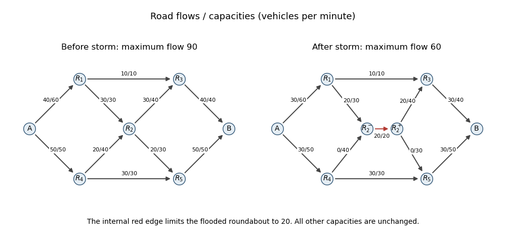
For the original roads, a feasible maximizing flow is given below; every table entry is flow/capacity in vehicles per minute.
| Road | Before storm | After storm |
|---|---|---|
All road capacities are respected, and direct summation verifies flow conservation at each roundabout. The original flow value is . The cut separating from every other vertex consists of its two incoming roads and has capacity . Therefore the original maximum is 90 vehicles per minute.
To impose a vertex capacity, split into and . Send its incoming roads to and its outgoing roads from , and add a directed internal edge of capacity . Every unit passing through the roundabout must traverse this internal edge. This gives the standard maximum flow with vertex capacities construction.
Starting from zero, apply the Ford-Fulkerson algorithm with the following augmenting paths in order. First use : its residual capacities are , so augment by . Next use : the residual capacities are , so augment by . Finally use : the residual capacities at this stage are , so augment by . No reverse edge is needed in this valid run. The resulting original-road flows are precisely the after-storm column above, and the internal edge carries .
For termination and optimality, take the source-side set . Its outgoing edges are , and , of capacities . They are all saturated, and no positive-flow original edge enters this set. Consequently no residual path leaves the set, and its cut capacity equals the constructed flow value. The new maximum is therefore
Articles by others on the same topic
There are currently no matching articles.