Original source: Original released paper, physical PDF pages 120–127. All questions and all three D13 alternatives are covered.
For a lossless antireflection coating, cancellation requires both equal reflected wave amplitudes and an odd half-cycle difference in their round-trip wave phase. At normal incidence the interface amplitude coefficients are and . Choosing makes both negative: both reflections acquire the same phase reversal. A quarter-wave optical thickness supplies their remaining relative phase .
Equal amplitudes require , which reduces to . ThusThe exact multilayer reflection amplitude is zero for these choices, not merely the sum of the first two reflected rays: its numerator is , with . Any positive odd multiple of this thickness has the same cancellation at the design wavelength; the smallest is the thin-layer choice. absorption, index dispersion, angular spread and deviations from the selected wavelength limit the practical cancellation.
A Fresnel zone plate replaces a conventional refracting surface by concentric alternating transmitting and absorbing annuli. Successive annuli span half a wavelength of optical-path excess to the chosen focus; blocking alternate zones prevents their approximately opposite wave phases from cancelling. For a normally incident plane wave,The paraxial radii grow as , so the zones become narrower outwards.
Using the photon energy relation gives . For ,The first three boundaries are approximately , and . This fixes the zone pattern but does not fix a unique outside diameter: the number of zones is a design choice. For example, gives radius , diameter and outermost zone width about . A larger usable diameter requires finer outer zones.
One could pattern absorbing metal annuli on a thin X-ray-transparent support, choosing absorber thickness from its attenuation at the selected photon energy; that thickness cannot be determined from energy and focal length alone. The design is chromatic: for fixed radii , so a narrow energy band is needed for a sharp common focus.
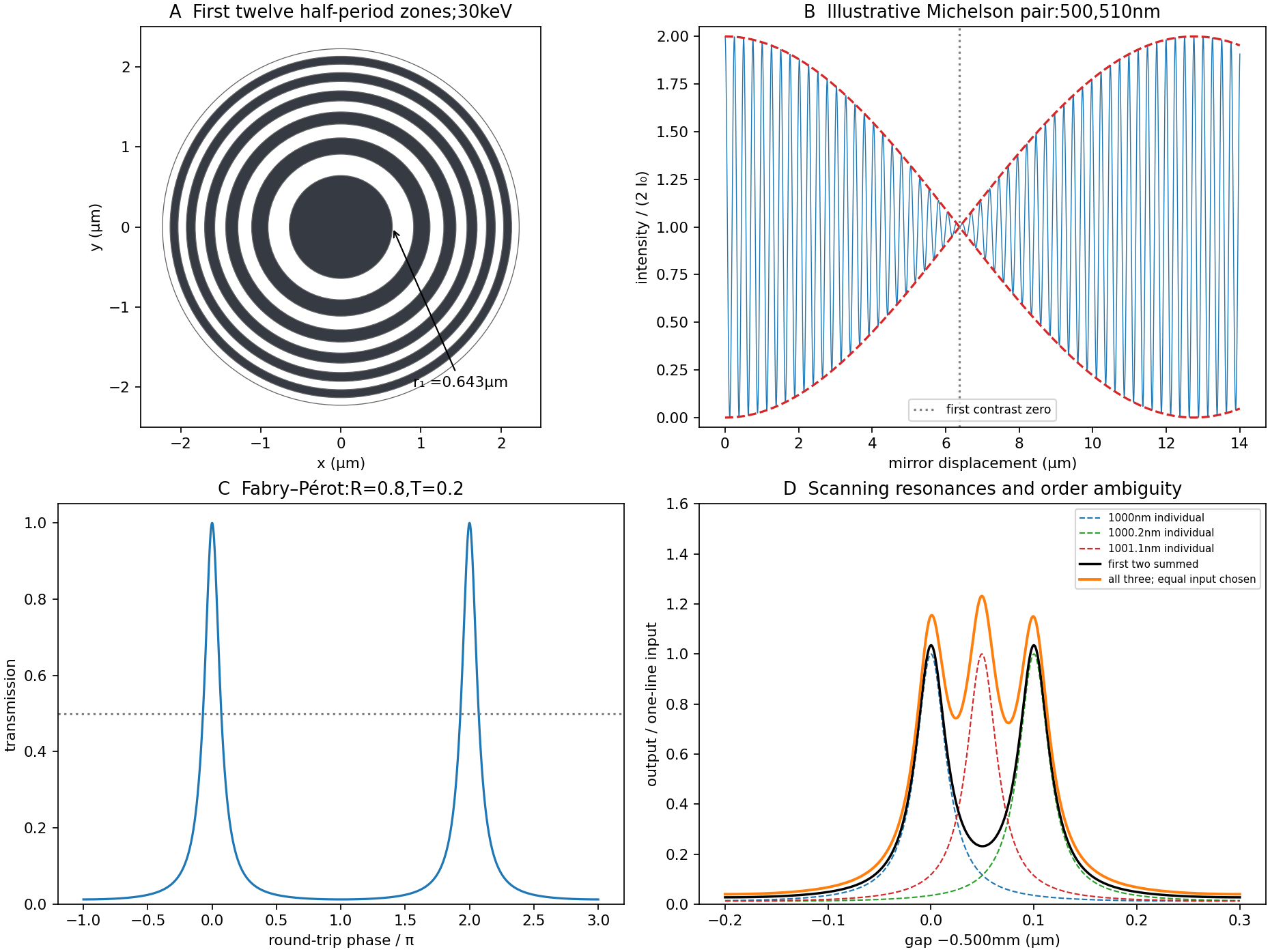

Let be mirror displacement from equal optical paths in a Michelson interferometer, so the optical path difference is . Different spectral components add detected light intensities; each component interferes with its own delayed copy. For equal line strengths and ideally balanced arms, writeThe trigonometric identity for the sum of cosines givesThus the sketch consists of rapid fringes within a slowly varying contrast envelope. With the mean wavelength and , the mirror-displacement fringe spacing is . The interference visibility isThe first contrast zero is at ; successive visibility maxima are separated byBetween successive contrast zeros the signed envelope changes sign, shifting the rapid fringes by half a cycle. Unequal line strengths leave a nonzero minimum contrast. Finite linewidth adds a longer-range coherence envelope, while arm imbalance and polarization mismatch can reduce contrast without indicating a different spectral spacing.
Use periodic boundary conditions temporarily to count the allowed wavevectors. Each state occupies in reciprocal space. For one acoustic polarization, the spherical shell between and containsBoth positive and negative wavevector directions are already included in that sphere; no further factor of two is needed. With the linear dispersion relation ,A three-dimensional monatomic crystal has three acoustic branches. Under the stated common-speed approximation,This is a phonon density of states per unit angular frequency, not per unit ordinary frequency. If longitudinal and transverse speeds differ, the isotropic expression becomes . In the Debye model, imposing sets the cutoff; the linear approximation is not continued to arbitrarily high frequency in a finite lattice.
The effective mass follows from the curvature of the electronic band structure. Differentiating twice givesAt either first Brillouin zone boundary ,The boundary is a band maximum, with negative curvature and zero group velocity. In the semiclassical single-band description, an applied force changes ; the resulting acceleration is opposite the force near that maximum. This is a band-response coefficient, not a negative microscopic electron rest mass. A nearly filled band is often described more conveniently through positively charged electron holes near its maximum.
Put and . The characteristic roots are . For release from rest at displacement , the three regimes areunderdamping produces decaying oscillations; critical damping is the repeated-root boundary; overdamping has two real decay rates. The critical and overdamped curves from rest approach equilibrium without crossing it. All three initially have zero slope and negative acceleration. A sufficiently strong initial kick can cause a single crossing even without an oscillatory mode.
For the critical oscillator with initial velocity , the repeated-root solution isIts exponential is positive at finite time. Therefore the bracket has a positive-time zero precisely whenEquality gives a pure positive exponential and no finite-time crossing.
For the specified numerical oscillator, and , verifying overdamping. Its two roots are and in inverse seconds. The initial conditions givewith in seconds. The slow component has a negative coefficient; the fast positive component initially dominates.
The values for the requested plot areThe curve crosses near and then returns toward zero from below. The exact expression provides a check on the graphical estimate:
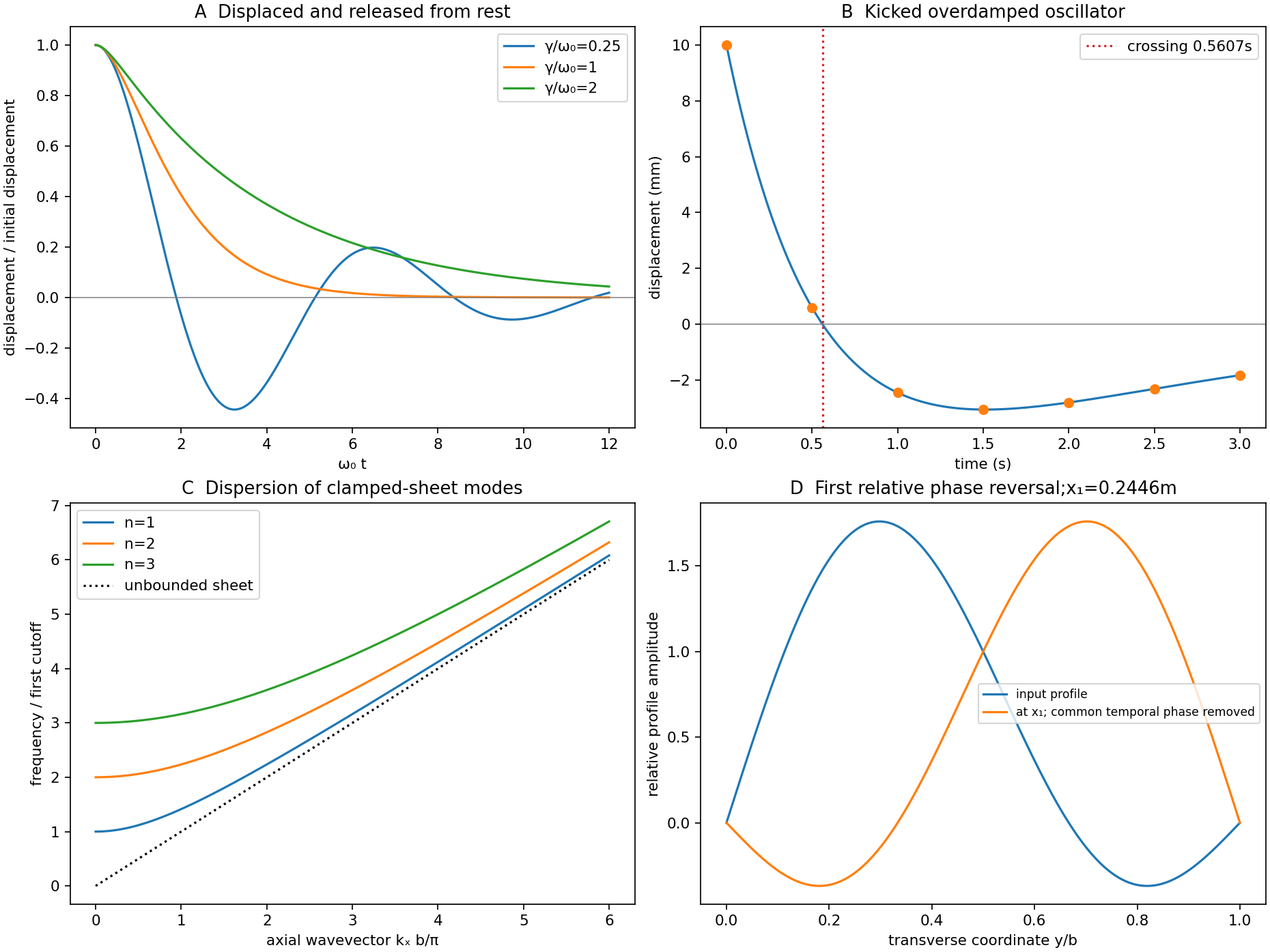

For a uniform taut sheet in the small-displacement approximation, the two-dimensional wave equation isSeek a harmonic solution . The clamped edges impose Dirichlet boundary conditions . Hence has nontrivial solutions only forTaking the real part gives the stated sinusoidal transverse profile. There is no nonzero mode satisfying both clamped boundaries.
Substitution gives the dispersion relationThe three branches have cutoffs at and approach at large . Only frequencies above a branch's cutoff give traveling waves along an infinitely long guide; below it, the axial dependence is evanescent. For a forward propagating mode,The phase velocity exceeds , while the group velocity is smaller: the carrier phase speed is not the signal speed.
Here the first two cutoff frequencies are and , so both modes propagate at . With ,Each transverse mode independently acquires its axial phase. The second mode first changes sign relative to the first when , givingAt that distance a common temporal phase is modulo ; the second term is negative relative to the first for every and every time, not just at one selected instant.
In an optical fibre, different guided modes have different group velocities, so an input pulse becomes a sum of differently delayed pulses. This intermodal dispersion broadens pulses and can make adjacent digital symbols overlap. A single-mode optical fiber removes this particular mode-delay mechanism; a graded-index optical fiber can reduce it in a multimode design. Single-mode propagation still permits wavelength-dependent group delay, so it does not remove every kind of optical dispersion.
The Fourier expression is the scalar Fraunhofer diffraction approximation for coherent, effectively monochromatic illumination with a uniform incident plane wave over the aperture. At a distant screen the aperture-dependent quadratic propagation phase must be negligible, roughly for transverse size . Alternatively, a thin lens forms the angular Fourier transform in its back focal plane. That focal-plane construction is the appropriate one here; the aperture-to-lens distance need not itself be an enormous free-propagation distance. aperture features should be large compared with wavelength for this simple scalar transmission-mask model.
If complementary transmissions are and , linearity gives . Away from the undiffracted forward beam, the uniform plane-wave contribution vanishes in angular space, so and their intensities agree. This is Babinet's principle. It equates the off-forward diffracted intensities, not the transmitted power or the on-axis intensity including the direct beam.
Let be screen coordinates conjugate to aperture coordinates , so , . With width along and height along , define . The complementary rectangle has transformThus the obstruction's off-forward scattered component hasIts dark lines occur atThe central-lobe zero-to-zero size is by ; it is wider in the direction conjugate to the narrower obstruction. The central forward image of the illuminating beam must be distinguished from this scattered envelope in a real screen observation.
The source figure gives centre-to-centre separation . Choose the three rectangle centres at ; an overall translation changes only the transform phase. Their scattered amplitude is proportional toThereforeAlong the screen's direction, the three-element interference factor has principal maxima separated by , under the single-rectangle envelope. Its zeros lie at and . It also has weaker secondary maxima between principal orders. Every fifth principal order coincides with a single-rectangle zero and is missing; multiplication by the envelope slightly shifts maxima away from the nominal interference-factor positions. The figure plots the calculated scattered component and marks the separate direct-beam limitation.
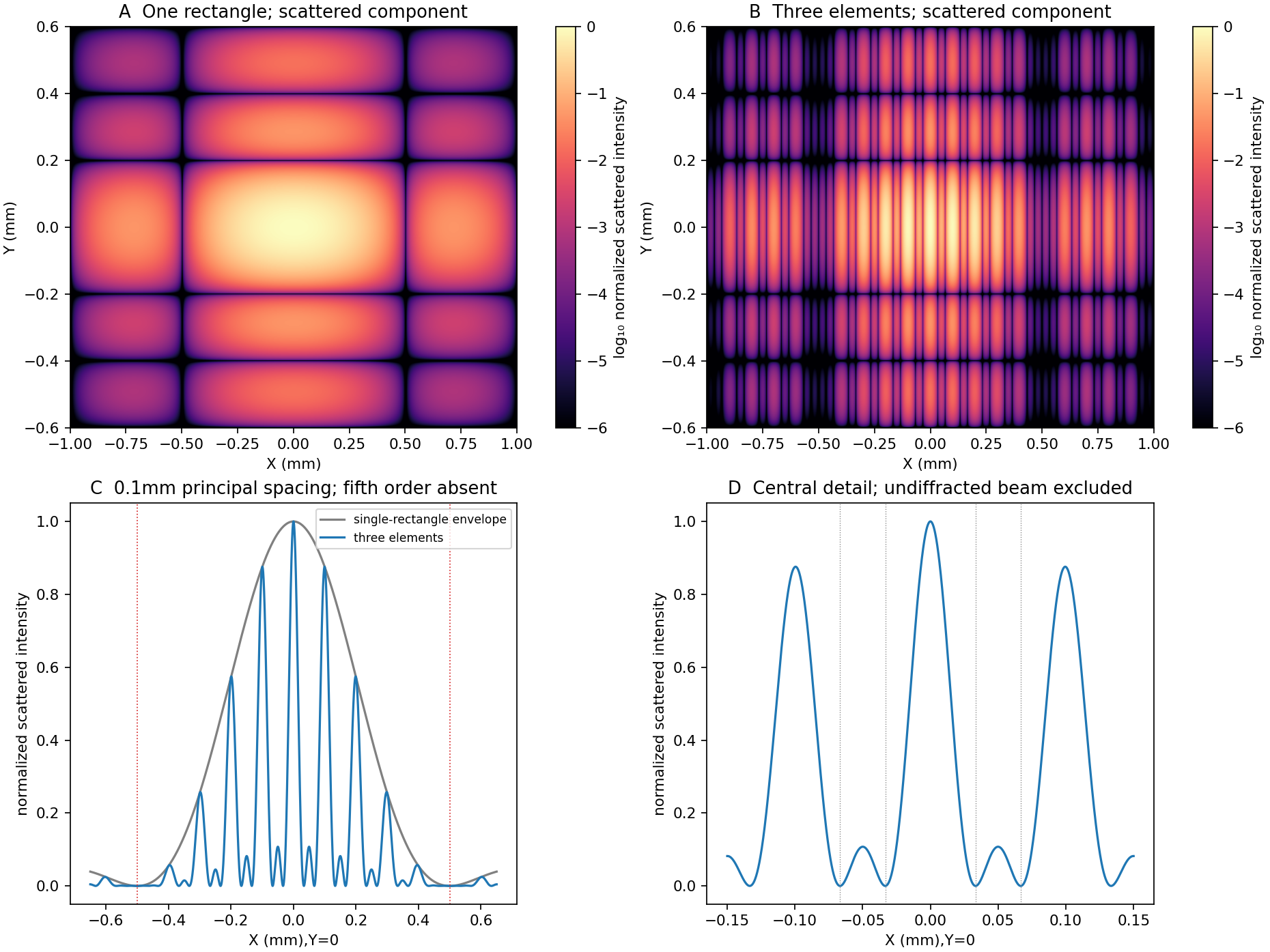
Original calculated rectangular-obstruction and three-element Fraunhofer scattered intensities
. Screen coordinates are physical conjugates of the obstruction coordinates. All plotted values describe the scattered component; the unresolved undiffracted illumination at the origin is excluded. Intensities are normalized, and no source figure is reproduced. Details.
Let the first transmitted complex amplitude be : two amplitude transmission factors each of magnitude give magnitude . Each extra internal round trip adds two amplitude reflections, with combined magnitude , and phase . With the mirror phase convention already incorporated in the stipulated ,Taking the squared modulus givesIt is , not , that multiplies the field after a round trip; would be the corresponding round-trip intensity fraction.
At resonance , . If is the positive phase displacement to half maximum,For , the stipulated high-reflectivity approximation gives , while the exact value is . The full width is twice this value. With , , and the pattern repeats every . Its ideal finesse is approximately .
A wavelength component resonates at . Within the scan interval, the individual resonances areNo neighboring orders of these lines fall within the stated interval. The observed signal is the sum of their two Airy transmissions, since different spectral components add intensities. Individual resonance positions identify the two peaks to the plotted precision; the tails cause very small shifts of the maxima of the sum.
The gap-coordinate full width isThe separation is , about full widths, so the two components can be resolved by the ideal etalon. The equivalent wavelength resolution near order is about , smaller than their separation.
The added wavelength has an order- resonance atIt lies between the preceding two peaks; its adjacent orders are outside the scan. Its input strength was not specified, so the third peak's height cannot be uniquely assigned. The original plot uses equal strength only as a declared illustration.
This is an order-identification problem: the free spectral range near is . A line more than one free spectral range away can appear among peaks of another order. A lower-resolution prefilter or additional dispersive spectrometer is needed to identify the order; a narrow peak alone does not identify an absolute wavelength. mirror parallelism, beam collimation and detector angular acceptance must also be controlled before attributing a measured width entirely to reflectivity.[ref]
Fabry-Perot Interferometer, University of Washington Physics 331. pp.2–5, instrument finesse and free spectral range; central-spot scanning discussion
Take the electron's signed charge to be , where is the elementary-charge magnitude. Conventional electric current flows along , while the mean electron drift velocity is negative. With , the magnetic Lorentz force separates charge across the width until a transverse electric field balances it. The accumulated edge charge then sustains a Hall voltage without a transverse steady current. In a one-carrier model, the Hall coefficient identifies the sign and number density of carriers; real multiband materials require a more careful interpretation.
The acceleration term contains the effective mass describing the local band response. The relaxation term removes drift momentum on the mean momentum-relaxation time . The remaining two terms are the electric and magnetic Lorentz force on signed charge ; the magnetic force is perpendicular to velocity and does no instantaneous work. The relaxation-time approximation replaces individual scattering events by an averaged drift equation.
Let be the electron number density, distinct from the negative charge . In transverse open circuit and . The steady component equations givehenceConsequentlyThere is no sign ambiguity in this field-defined once axes and carrier charge are fixed.
A measured voltage ratio additionally needs probe polarities, which the geometric bar diagram does not label. To reproduce the positive ratio specified for electrons, define the longitudinal voltage drop and the transverse rise . ThenReversing either voltage's probes reverses the measured ratio, without changing the physical carrier density. With both voltages instead defined as drops along their positive axes, the algebraic ratio would have the opposite sign. The figure records the convention used here.
A monovalent copper model assigns roughly one delocalized conduction electron per atom to a broad, approximately free-electron-like band. Using is therefore a sensible first estimate for its transport scale. Monovalence alone does not prove that every band curvature or orbit has exactly the free mass: periodic-potential mixing, the nonspherical Fermi surface and direction-dependent scattering limit the model. The calculated is conditional on the stipulated effective-mass approximation.
Experimentally, reverse both current and magnetic field and extract the part of the transverse voltage odd in each. This rejects fixed contact offsets and much longitudinal pickup; use four-terminal longitudinal sensing, measure dimensions independently and check heating before assigning material parameters. These controls are implemented in a reusable Hall/conductivity teaching experiment, although that experiment uses germanium rather than the copper sample here.[ref]
The Hall Effect and Conductivity in Germanium by Rex Tayloe. pp.1–3, equipment, contact geometry, room-temperature conductivity and four current/field polarity combinations
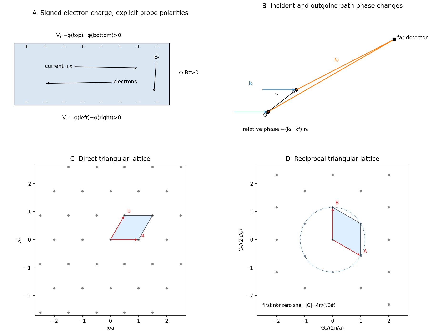

The reciprocal lattice consists of all wavevectors whose plane-wave phase is unchanged under every direct-lattice translation :It expresses periodicity in wavevector space, with dimensions of inverse length.
Choose incident field convention . The wave at the second atom acquires incident phase relative to the atom at the origin. Its path to a distant detector is shorter by approximately , contributing outgoing phase . ThereforeNeglecting variation of detector distance across the specimen, identical atoms have a common scattering amplitude factor andThe original geometry diagram shows the incident direction, outgoing direction and direct-space displacement separately; is a wavevector difference, not an extra ray path.
The primitive reciprocal vectors obeywith cyclic versions for . If , every lattice term has phase times an integer, so all terms add constructively. Conversely, full translational reinforcement requires , and to be integer multiples of , hence is reciprocal. These are the Laue equations. A finite crystal gives finite-width maxima rather than ideal reciprocal-space delta peaks; elastic scattering must also satisfy .
For the two-dimensional Bravais lattice interpretation, with one atom per primitive cell, takeSolving the duality conditions givessoThe reciprocal primitive vectors have equal length and angle ; the array itself is triangular. A different primitive basis can use a angle without changing the lattice. The direct primitive-cell area is and its reciprocal-cell area is divided by that area.
For nonzero integer pairs, has minimum one, attained for six shortest vectors. Therefore the first nonforward maximum has . If the forward transmitted maximum is included literally, the smallest value is ; the nonzero value is the first diffraction shell. Reaching that shell in elastic scattering additionally requires .
Fresnel diffraction is interference during propagation when curvature of the optical path across an aperture matters. It provides a continuous account of fringes near geometric edges and their evolution into the far-field pattern. A screen that is many aperture widths away is not automatically in the Fraunhofer diffraction limit; wavelength also enters the comparison.
For plane-wave illumination of a transmission at , the Huygens-Fresnel principle in the scalar paraxial approximation givesIt follows by expanding the propagation distance as while treating the amplitude prefactor as slowly varying. Small propagation angles justify dropping higher path terms. Finite coherent illumination, vector edge fields and very small apertures can require a more complete theory. The Fresnel number , with a clearly declared aperture scale , measures whether the aperture's quadratic phase is significant. When it is negligible, the remaining linear phase produces the aperture Fourier transform.[ref]
Interactive Optics by Sander Konijnenberg, Aurèle J.L. Adam and H. Paul Urbach. Scalar Diffraction Optics, Fresnel Approximation and Fresnel and Fraunhofer Approximations, equations381–392
Define the optical Fresnel integralsTheir limiting values are , with odd continuation to negative arguments. The Cornu spiral plots : the field contributed by a finite interval is proportional to the chord between its endpoints. Intensities require squared chord lengths; summing zone intensities would lose the cancellation mechanism.
For an opaque straight edge transmitting and all , let , so is the geometrically illuminated side. Integrating in the unrestricted transverse direction and using the half-line in the other giveshenceFar into the shadow, ; far into the illuminated region, . At the geometric shadow boundary, , not half the incident intensity: the field is halved there. On the illuminated side, alternating constructive and destructive contributions give bright and dark fringes whose contrast declines away from the edge. Their positions scale with and are not equally spaced. A finite detector averages fine fringes and tends to recover the geometric-optics step. In a controlled experiment, translate a straight edge through a broad collimated beam, scan a small photodetector across the screen and normalize against an unobstructed reference; vary to test the square-root scaling. Source size, spectral bandwidth, edge roughness and detector aperture wash out contrast and must be distinguished from a failure of the propagation law.
For a rectangular aperture of full widths , defineThe two transverse integrals separate:andA long slit leaves only one varying Fresnel factor. For a square centred on axis, and giveOpposite edge contributions overlap; changing aperture size or propagation distance changes their relative phase. Consequently a geometrically illuminated centre can brighten or darken, rather than remaining a fixed top-hat plateau. The original rectangular-aperture map shows fringes parallel to both edges and their crossing structure. Outside the geometric rectangle the wave also extends into the shadow.
At large Fresnel number an interior region approaches geometric illumination while edge fringes remain on a scale . At intermediate values the opposite-edge fringes interact across the whole aperture image. In the far field, the formula tends to the product of sinc-squared factors,The far-field lobe scale grows linearly with , unlike the local near-edge scale. The transition is controlled by the neglected phase, not an abrupt physical boundary.
To test the main effect, record normalized profiles at several distances, calculate the Fresnel integral with the measured aperture dimensions and compare fringe positions before fitting a free intensity scale. Use the same transverse coordinate origin and check that the incident beam is sufficiently uniform. Babinet's principle relates complementary aperture and obstruction fields through ; their near-field intensities are not generally equal, because the unobstructed field remains present and interferes with the diffracted field. This is why a far-field obstruction argument cannot simply be carried over as equality of Fresnel intensities.
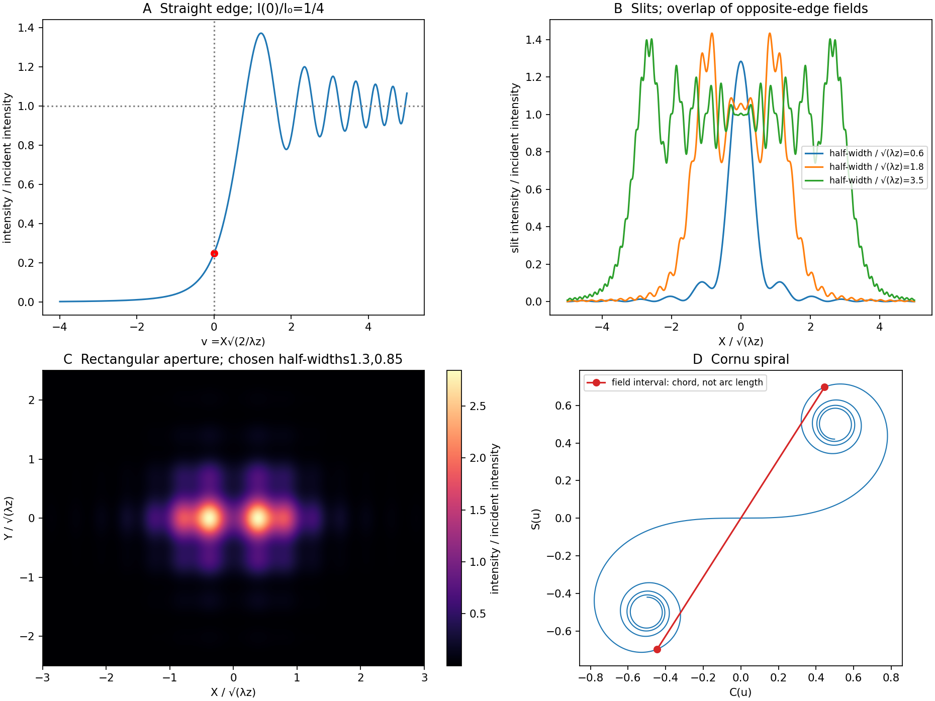
Original Fresnel-integral calculations for a straight edge, slits, rectangular aperture and Cornu spiral
. The plots use the stated scalar paraxial model and chosen dimensionless aperture parameters. The straight-edge boundary value is one quarter. The aperture panels show quadratic-phase propagation and the Cornu panel identifies field amplitudes as chords rather than summed intensities. Details.
The free electron model replaces the detailed periodic potential by a constant background, treating conduction electrons as mobile particles with approximately parabolic dispersion . It is useful to distinguish the classical Drude model from the quantum free electron gas. They share a simple transport picture, but differ fundamentally in occupation statistics.
With a momentum-relaxation time , both lead in a simple isotropic one-band approximation toThis explains approximately Ohmic longitudinal conduction and a carrier-density scale from the Hall effect. The relaxation time is phenomenological: introducing it does not itself predict scattering from defects or phonons. A four-probe resistance measurement separates the sample's longitudinal response from current-contact voltage drops; field and current reversals isolate the transverse signal.
The classical model incorrectly assigns roughly of electronic heat capacity, far too large in a degenerate metal. Fermi-Dirac statistics fixes this: most occupied states cannot change occupation after a small thermal perturbation because nearby low-energy states are already filled. Only a fraction of order near the Fermi energy participates. For ,The quantum model also gives a finite Fermi velocity even at zero temperature and Pauli paramagnetism. Under predominantly elastic scattering, its electronic heat and charge conductivities obey the Wiedemann-Franz law,This is a quantum success; classical equipartition does not give the correct small heat capacity and Lorenz number together.
Its limitations are equally instructive. Without the periodic potential it has no band gaps, so it cannot distinguish a filled-band insulator from a metal or explain semiconductor doping. The simplest single-electron Hall formula cannot explain positive Hall coefficients; band curvature and electron holes, or a multiband transport treatment, are needed. It neglects much Fermi-surface anisotropy and detailed optical interband absorption. Noninteracting electrons alone do not explain ferromagnetism or superconductivity, and lattice thermal behavior needs phonons. The nearly-free electron model, which allows reciprocal-lattice Fourier components of the potential to mix plane waves, provides a controlled first correction near Bragg planes.
Its main success is a simple quantitative baseline for degenerate conduction electrons; its main failure is treating the crystal and interactions as too featureless. A fit of conductivity alone is not a test of the whole model: compare heat capacity, Hall sign, optical response and temperature dependence using independently constrained parameters.
In an electrical insulator, lattice vibrations usually carry most heat. A small temperature gradient produces an imbalance between phonons moving in opposite directions. In an isotropic kinetic approximation,where is heat capacity per unit volume, an appropriate acoustic speed and the transport mean free path. The factor one third is the angular average of the squared direction cosine. With several branches and frequency-dependent scattering, replace this estimate by the corresponding weighted mode integral. A short lifetime matters for conductivity only insofar as it relaxes heat current.
For a clean three-dimensional crystal at , the Debye heat capacity varies as . If diffuse boundary scattering fixes near a specimen dimension, then . The size dependence is a test of that boundary-limited regime. Specular surfaces, defects and small specimens can change the simple law; at ballistic scales a local conductivity description itself needs care.
As temperature rises, more phonons are excited, but phonon-phonon scattering shortens their transport path. Normal processes conserve total crystal momentum, whereas an Umklapp process satisfies with reciprocal vector and can relax directed heat flow. Low-temperature Umklapp scattering is strongly suppressed; its increasing importance often produces a conductivity maximum followed by a decline. Isotope and impurity scattering lower or broaden that maximum.
At sufficiently high temperature, approaches its classical constant while a typical anharmonic Umklapp rate grows approximately as . Under that further approximation,Thus a clean crystalline insulator commonly shows a low-temperature rise, a peak, then a high-temperature fall. This is not a universal curve for every insulator: glasses, strong disorder, multiple scattering mechanisms, radiative heat transfer and structural transitions can give different behavior.
A steady-state bar experiment supplies a concrete test. Inject known heating power, measure the small temperature difference between two separated sensors and infer after correcting for heat leaks. Keep the gradient small enough that a single representative temperature is meaningful, calibrate sensor contact effects and subtract radiative/background losses. Repeat with different widths or isotope/defect content to distinguish boundary limitation from intrinsic scattering. A power-dependent result may reflect a changing temperature profile rather than a new microscopic law.
A p-n junction brings p-type and n-type regions into contact. Majority-carrier diffusion initially leaves exposed ionized acceptors and donors, producing a depletion region and a built-in potential. At thermal equilibrium the electrochemical potential is constant: drift and diffusion currents cancel. The internal barrier is not a freely extractable battery voltage.
For a nondegenerate abrupt homojunction,Here denotes forward bias and the depletion approximation is assumed. forward bias lowers the barrier and injects minority carriers; reverse bias widens the depleted region and suppresses ordinary majority injection. In the ideal diffusion regime,Recombination can change the ideality factor; series resistance, high-level injection, leakage and breakdown limit this simple Shockley diode equation. The original junction theory explicitly treats both electron and hole currents, which is essential to carrier injection and transistor action.[ref]
The Theory of p-n Junctions in Semiconductors and p-n Junction Transistors by William Shockley. 1949, pp.435–436, introduction: rectification, photosensitivity and injection of minority carriers
As a rectifying diode, the junction conducts strongly in one bias direction and weakly in the other before breakdown. This permits power rectification, signal detection and electronic switching. Stored minority charge affects turn-off time, so a static exponential current-voltage relation alone does not specify switching speed. A junction capacitance varies with reverse bias and can be used in a voltage-controlled capacitor; heavily doped or high-field junctions can instead exploit controlled tunnelling or avalanche breakdown.
In a photodiode, absorbed photons generate electron-hole pairs and the depleted-region field assists collection. reverse bias widens the collecting region and can improve speed, but adds dark-current noise and breakdown constraints. In a solar cell, the same carrier generation supplies current against an external voltage. An ideal illuminated characteristic is : at open circuit the forward diode current balances photocurrent, while useful power is taken at an intermediate operating point. Neither short circuit nor open circuit delivers power to a load.
A forward-biased light-emitting diode injects electrons and holes that can recombine radiatively. Efficient emission favors suitable direct-gap materials and carrier confinement; the characteristic photon energy is near the semiconductor band gap. nonradiative recombination, escape losses, series resistance and heating limit efficiency. Two coupled junctions also form a bipolar junction transistor: an emitter injects minority carriers through a thin base, and a reverse-biased collector collects them. Useful current gain depends on efficient injection and limited base recombination, not simply on joining any three arbitrary regions.
These functions are experimentally distinguished by measuring dark and illuminated current-voltage curves, bias-dependent capacitance, transient switching or optical emission, with controlled temperature and current limits. The common mechanism is bias-controlled carrier injection or collection at a depletion barrier; the device geometry and operating mode determine which function is useful.
Articles by others on the same topic
There are currently no matching articles.