The original cover dates this examination to 22 June 2015, 9.30–11.00am. The archive stores it under
2014/T/a13752w1.pdf; the cover determines the year. Source: released examination archive.The intact copy in the Mathematics Part A release, member
FOI-20210708-1 - Data/a13752w1 (4).pdf, restores the previously missing printed page 3 and supplies a complete readable counterpart. Questions 1–2 had already been recovered and answered; those answers and all answers to questions 5–8 are retained. The solutions now cover all eight questions and their 37 leaf subparts. The earlier source provenance above is unchanged.The binomial theorem isolates the only terms that can survive reduction modulo the prime number :For , neither nor is divisible by , whereas is. Consequently , and every intermediate term vanishes in modular arithmetic. ThusThis works for arbitrary integers , including those divisible by . It is the additive identity behind the Frobenius endomorphism in characteristic .
For an odd prime number , Euler's criterion states thatwhere the Legendre symbol is zero if , one if is a nonzero quadratic residue, and minus one otherwise. Including the zero case makes this formulation valid for every integer .
Apply Euler's criterion to , , and . Multiplication in modular arithmetic givesIf divides either factor, both sides are zero. Otherwise both sides belong to ; these two values are distinct modulo the odd prime number . The congruence is therefore an equality of integers, proving multiplicativity of the Legendre symbol:
For distinct odd prime numbers , the law of quadratic reciprocity isThus the two Legendre symbols agree unless both prime numbers are congruent to modulo , in which case they have opposite signs.
In Pollard's p-1 algorithm, a large exponent containing many small factors makes divisible by a prime factor whose predecessor divides , by Fermat's little theorem. A greatest common divisor with the number being factored can then separate that prime factor from the others.
Choose base and build factorial exponents using modular exponentiation. The successive exponents , , and giveThe first two greatest common divisors are . At the next step the Euclidean algorithm givesHenceHere the element order of modulo is , which divides , even though does not divide . The algorithm only needs the element order to divide the chosen exponent; divisibility by the full predecessor is a sufficient condition, not a necessary one.
First simplify the specified residue by modular exponentiation. Modulo the prime number ,Therefore , so the required equation becomes . Its right side is nonzero, so any solution is a unit modulo .
By Fermat's little theorem, exponents of such units can be reduced modulo . Sinceraising to the th power is the inverse of raising to the th power. There is therefore exactly one residue class of solutions:Now and . Since , we obtainAs a direct check, , , , and , whence .
The defining relation lets us move every occurrence of to the right of every occurrence of . More generally, repeated conjugation givesNegative powers cause no problem because and . Thus every word in the group presentation can be put in the required form, reducing powers using :At this stage existence is proved; uniqueness will follow from the concrete semidirect product in part (b). Moving past gives the multiplication lawThe action is consistent with reduction of modulo because .
For the given group homomorphism , the external semidirect product has underlying Cartesian product and operationThe notation denotes the automorphism group of . Closure follows because is an automorphism of . To check associativity, calculate both bracketings:They agree because . The identity is , using , and the two-sided inverse isIndeed multiplication in either order gives the identity, using . This verifies the group axioms.
For the specified group presentation, take and . The rule defines an automorphism because is coprime to . Furthermore , so defines the required group homomorphism . In the resulting semidirect product , the canonical generators satisfyConsequently the group presentation defines a surjective group homomorphism , sending to and to . The underlying Cartesian product gives , whereas part (a) gives . Surjectivity forces equality, so the map is an isomorphism:This also proves that the normal forms in part (a) are distinct and that has element order exactly .
The cyclic subgroup is normal: conjugation by sends to , and conjugation by fixes it. Modulo this subgroup, the relation becomes , so the quotient group is Abelian. Thus the commutator subgroup is contained in .
Conversely the displayed relation gives the commutator , so . HenceSince has element order , , so the first commutator subgroup is nontrivial. ThereforeHere derived length counts the number of steps needed for the derived series to reach the trivial group.
The given unitriangular group of degree three over F3 has elements, just as does, so counting alone cannot distinguish them. Instead compare element orders.
Write an element as , with strictly upper triangular of size . Then . Over the finite field , the binomial theorem for commuting matrices givesEvery nonidentity element of consequently has element order . In contrast, has element order , by part (b). An isomorphism preserves element order, soEquivalently, the exponent of a finite group is for and for .
Use the cross-ratio convention compatible with the permutation identities in this paper. Represent a projective point by a nonzero vector , and write . DefineThe denominator is nonzero because the four projective points are distinct. Rescaling any one representative multiplies numerator and denominator by the same nonzero scalar, so the definition is independent of the chosen homogeneous coordinates. In finite affine coordinates it readswith the point at infinity of the complex projective line handled by the homogeneous formula.
A projective transformation is represented by an invertible matrix . Since , the two factors of in the numerator cancel the two in the denominator. Therefore every projective transformation preserves this cross-ratio. This also shows that the formula descends from matrices to the projective linear group, whose representatives differ by a nonzero common scalar.
The needed general-position theorem is sharp triple transitivity of the projective linear group on the projective line: for any two ordered triples of distinct projective points, exactly one projective transformation takes the first triple to the second.
In particular, let take to . In these coordinates,so cross-ratio invariance gives , where . Distinctness implies and is finite. The entire ordered quadruple is thus normalized toFor a second quadruple with the same cross-ratio, its normalizing map yields the same quadruple. ConsequentlyThis proves the equivalence. Uniqueness on the first three points also shows that the projectivity carrying one ordered quadruple to the other is unique. The cross-ratio normalization of four projective points therefore gives a complete invariant for this ordered classification.
Choose three distinct projective points . Their images under the injective map are distinct. Sharp triple transitivity gives a projective transformation agreeing with on these three points. The map fixes and preserves their cross-ratios.
For any other projective point , invariance givesLet normalize to . By part (b), the left side is and the right side is . Since is a bijection, . It fixes the original three points too, so is the identity map everywhere. ThereforeNo continuity or prior surjectivity assumption was needed. This is the rigidity assertion that cross-ratio preserving maps are projective.
By invariance under projective transformations and part (b), it is enough to calculate on the normalized quadruple . Direct evaluation of the cross-ratio givesFor instance, , and . ThusAll denominators are legitimate because . The first identity explains why some distinct permutations always give the same cross-ratio.
The cross-ratio permutation orbit is generated by the two operations and from part (d). The full list isThese are all the possibilities: the four permutations generated by interchanging both pairs and by exchanging the two pairs leave the cross-ratio unchanged. They form the Klein four-group inside the symmetric group on four symbols, leaving at most different values; the displayed operations attain all six rational expressions.
There are fewer than six values exactly when a nonidentity operation in this six-element action fixes : if two operations give the same value, composing one with the inverse of the other gives such a fixed point. For real , the fixed-point equations areThe other two equations reduce to , which has no real root. HenceEach exceptional value has the same three-element orbit . Every other permitted real value gives six different values.
For the geometric interpretation, put and for . ThenThe three exceptional cases becomeThus the three finite points are collinear and equally spaced, with one their midpoint, even when the are viewed as points of the complex plane. Equivalently they form an arithmetic progression in some order. These are the harmonic conjugate points configurations with the fourth point equal to the point at infinity of the complex projective line.
A map is differentiable at when a linear map approximates its increment to first order:This Fréchet derivative is unique, and its matrix in the standard bases is the Jacobian matrix. Differentiability on a domain means differentiability at each point there.
A standard sufficient condition for a zero locus to be a submanifold is the regular level set theorem: if is on an open domain and is surjective at every , thenFor smooth , the submanifold is smooth. The full-rank condition is the relevant constraint qualification.
Under this regularity hypothesis, its tangent space isIndeed, if a differentiable curve lies in and passes through , the chain rule gives . Thus all tangent velocities lie in the kernel of a linear map. The rank-nullity theorem makes this kernel -dimensional, the same dimension as the tangent space, proving equality. In coordinates, solve the homogeneous linear equations given by the Jacobian matrix.
The regularity qualification matters: has zero set , a zero-dimensional submanifold, but . Its kernel is all of , whereas its tangent space is zero. This is the phenomenon that singular defining maps can overestimate tangent spaces.
At a constrained critical point, the directional derivative of vanishes along every admissible tangent velocity:For a regular zero locus, . A linear functional vanishing on this kernel lies in the row space of . Equivalently there are Lagrange multipliers such thatGeometrically, is orthogonal to the tangent space, so it lies in its orthogonal complement, spanned by the independent constraint gradients. Thus the level set of has no first-order change in a tangent direction. The equations provide candidates for constrained extrema; they must still be classified and compared, and boundary or singular cases must be treated separately. The condition is necessary for a regular constrained extremum, not a guarantee of a maximum.
The feasible set is closed and contained in the rectangleIt is therefore compact, and the continuous function attains a global maximum there by the extreme value theorem. At the two boundary endpoints where a coordinate is zero, the product is zero. Meanwhile is feasible because the conjugate exponents satisfy , and its product is one. Hence every maximizer has .
On that positive region the constraint is with nonzero gradient. The Lagrange multiplier equations areThe first two identities imply . Since , the multiplier is nonzero, so . The constraint now givesThus the sole interior candidate is . Existence of a maximum and the boundary comparison prove the unique global resultThis conjugate-power constrained product maximum is valid for all real with ; no integrality of the exponents is needed.
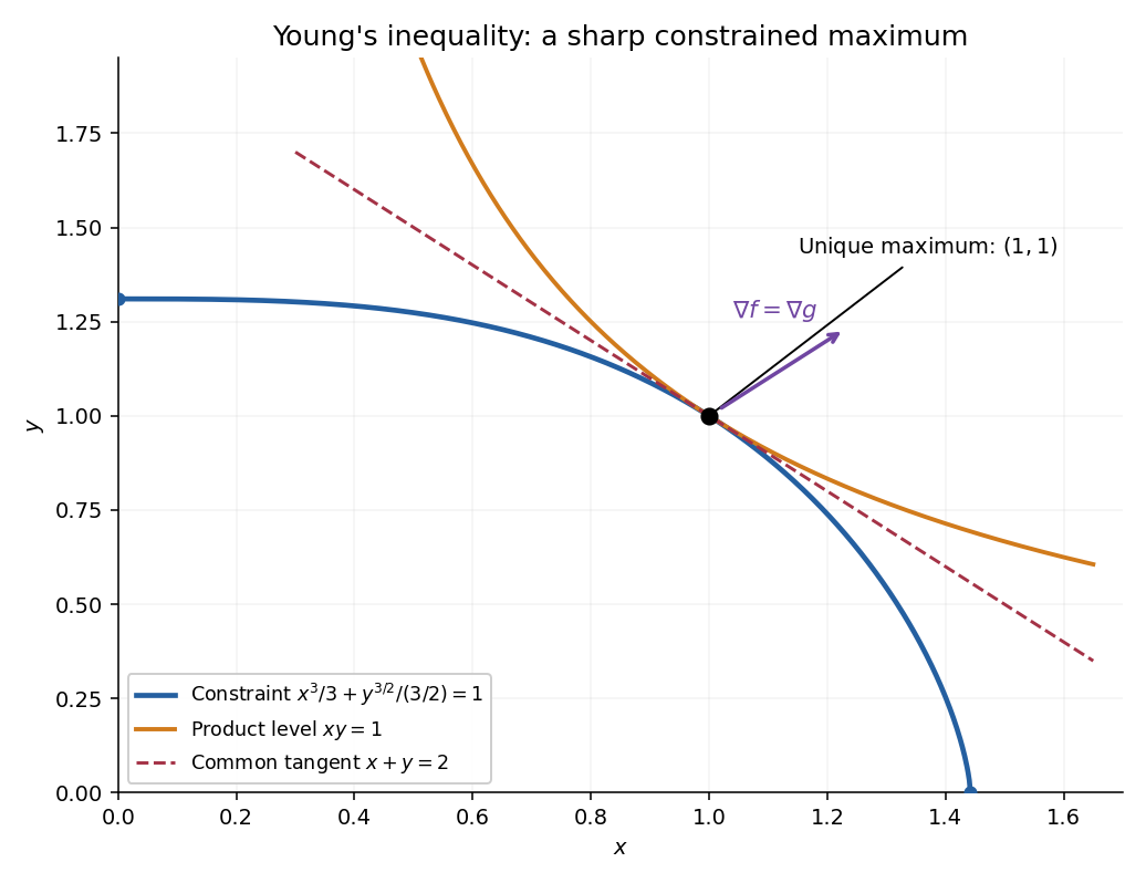
The constrained product reaches one where the two level curves are tangent
. Original illustration for p=3 and q=3/2. The constraint arc meets the product level xy=1 only at (1,1), where both gradients point along (1,1). The red dashed line is their common tangent. Details.
Use a normalization proof of Young's inequality. For arbitrary , putIf , both coordinates are zero and the desired inequality is equality. If , defineThen . Part (c) gives , and the conjugate exponent identity gives . Therefore Young's inequality for products isThe unique equality case in part (c) says . Translated back, and including the zero case, this gives the sharp conditionConversely, if both powers equal , then and the right side is , directly verifying equality.
Use the unilateral Laplace transform convention . The Laplace transform of a derivative isThe formula holds in the common Laplace convergence region under the usual endpoint and growth hypotheses. The initial value is the right-hand value at zero.
The defining evaluation rule of the Dirac delta givesThe impulse lies strictly inside the integration domain, so there is no endpoint convention to settle. This Laplace transform exists for every complex .
Let and . Apply the Laplace transform of a derivative twice and use the two zero initial conditions. The differential equation becomesThe factor is the Laplace transform of . The convolution theorem for Laplace transforms therefore givesThis is a causal convolution: the value at uses only the forcing up to . For ordinary continuous , direct differentiation gives and , verifying both the differential equation and the initial conditions. For an impulsive , the same formula is interpreted using distributions.
An impulse at shifts the causal sine response. Substituting the Dirac delta in the convolution from part (i), or using the Laplace transform time-shift rule, giveswhere is the Heaviside step function. The answer is continuous at , while its first derivative jumps from to . Consequently its second distributional derivative contains exactly one unit Dirac delta at , giving . Since , both initial conditions vanish.
Put , initially for real . Besides the Laplace transform of a derivative, use multiplication by the original variable in the formTransforming the Bessel differential equation, with its given initial conditions, yieldsThe constant terms cancel, leaving . This first-order ordinary differential equation integrates toThe initial value theorem for Laplace transforms gives , so . Thus the Laplace transform of the Bessel function J0 isFor complex with , choose the analytic square-root branch agreeing with the positive square root on the positive real axis.
For the forcing , part (b) now gives . On the other hand, the same multiplication rule givesTaking an integral from zero divides the Laplace transform by . By uniqueness of the Laplace transform,A direct check also explains the cancellation. This expression has and . The Bessel differential equation says , so integration from zero gives . Hence , and both initial conditions hold.
Use the chain rule along a sufficiently smooth extremal of the functional. For ,The bracket vanishes by the Euler-Lagrange equation. When has no explicit dependence, , giving the Beltrami identity:
For the specified functional,Since , the Beltrami identity gives for some . This suggests a circular arc, but it is worth deriving its equation without dividing by : such division would lose the point where the arc is horizontal.
Substitute the displayed partial derivative and in the full Euler-Lagrange equation. Combining terms over the common denominator givesThus , so and a second integration givesThis establishes the semicircular extremals of the hyperbolic length functional and excludes constant , which would satisfy the first-order Beltrami identity for a suitable but not the full Euler-Lagrange equation.
The two prescribed endpoints giveSubtracting yields . ThereforeIn particular the centre is . Admissibility requires , as the prescribed heights must lie in . Under that condition the radicand is positive throughout : it is a concave quadratic polynomial whose two endpoint values are and . The positive root consequently gives one smooth admissible arc, uniquely determined by the endpoints.
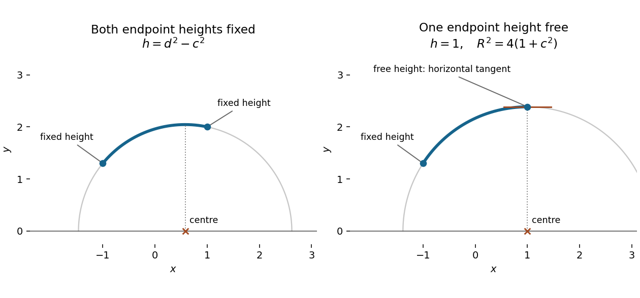
Fixed endpoint heights determine the circle centre; a free endpoint height forces a horizontal tangent
. Details. 
When an endpoint's horizontal coordinate is fixed but its height is free, the natural boundary conditions for a free endpoint require there. In this problem,Every admissible extremal is an upper circular arc with centre on , by part (b). Its tangent is horizontal precisely above its centre. Thus imposing the natural boundary conditions for a free endpoint at forces . The fixed height at gives , soIts free endpoint height is . Positivity on the whole interval follows because the radicand is at least .
There can be no solution satisfying the natural boundary conditions for a free endpoint at both ends: an upper circular arc has only one point with a horizontal tangent, whereas the two endpoints have distinct horizontal coordinates. Therefore
A tree is a nonempty connected graph with no graph cycle. A leaf of a tree is a vertex of vertex degree one. As usual in this finite graph theory problem, trees are finite; the assertion would fail for a doubly infinite graph path.
Take a longest path in a tree with at least two vertices. Connectedness gives . If had a neighbour outside this graph path, the path could be extended, contradicting maximal length. If it had a neighbour with , that edge together with the segment would make a graph cycle. Thus its only neighbour is , and it is a leaf of a tree. The same argument at the other end makes a second, distinct leaf of a tree. Hence
Deleting a vertex and its incident edge cannot create a graph cycle, so is acyclic. It remains to establish connectedness and nonemptiness.
Since the leaf of a tree has one neighbour, has at least two vertices, so is nonempty. For any two remaining vertices , take their unique simple graph path in . It cannot pass through : an internal vertex on such a graph path has two incident edges, whereas has vertex degree one. Neither endpoint is , so the entire graph path remains after deletion. The remaining graph is connected and acyclic, givingThis includes the two-vertex case, where deletion leaves the one-vertex tree.
Here each is a nonempty connected subgraph of a tree, rather than a descendant-closed data-structure subtree. We prove the Helly property for connected subgraphs of a tree by mathematical induction on the number of vertices of .
For a one-vertex tree, every nonempty contains that vertex. For a larger tree, choose a leaf of a tree using part (i), and denote its unique neighbour by . If some consists only of , the assumed pairwise intersections force every to contain , and we are done.
Otherwise, remove from every that contains it, leaving all other unchanged. Any affected has at least two vertices; connectedness forces it to contain and the edge . Thus is a leaf of a tree of , and part (ii) shows that its deletion leaves a nonempty tree. All reduced are therefore nonempty connected subgraphs of a tree .
They still intersect pairwise. An original common vertex other than survives. If a pair had only in common, both members would also contain , by the previous paragraph, contradicting that it was their only common vertex. The induction hypothesis now supplies a common vertex of the reduced family, which is also common to the original family. Consequently
A matching in a graph is a set of edges no two of which share a vertex. A cover here means a vertex cover: a set of vertices such that every edge has at least one endpoint in . It is not an edge cover.
Kőnig's theorem for bipartite matching states that, in any finite bipartite graph, the maximum size of a matching in a graph equals the minimum size of a vertex cover:Here is the matching number and is the vertex cover number.
Choose a maximum matching and a minimum vertex cover . By Kőnig's theorem for bipartite matching, . Every edge of must have at least one endpoint in , because is a vertex cover. Distinct edges of the matching in a graph have disjoint endpoints, so these requirements already use at least distinct vertices of .
Since has exactly that many vertices, each edge of has exactly one endpoint in , and no vertex of lies outside the endpoints of . Thus selecting the unique endpoint in from each edge of produces precisely the vertex cover :The argument also covers an edgeless graph: take both sets empty.
For every matching in a graph and every vertex cover , the disjoint edges of need distinct covering vertices. ThereforeNow assume the assertion in part (ii). It supplies a matching in a graph and a vertex cover formed by choosing one endpoint of each edge of . Because these edges are disjoint, the chosen endpoints are distinct, so . By the definitions of maximum and minimum,Every inequality must be equality, proving Kőnig's theorem for bipartite matching:
Use coordinates and Minkowski metric . A real matrix is a Lorentz transformation precisely when it preserves the Minkowski interval for every , equivalentlyIt is proper when , and orthochronous when , equivalently . The latter selects the orthochronous Lorentz group, which preserves future-directed timelike four-vectors. Indeed the time-time entry of the preservation identity gives , so . Imposing both conditions gives a proper orthochronous Lorentz transformation.
Now use and . WritePreservation of the Minkowski metric says that the first column has squared norm , the second has squared norm , and the columns are orthogonal for the Minkowski inner product:Orthochronousness gives . From the orthogonality equation, ; substituting in the second norm identity gives . Hence with . The determinant is then , so properness forces . Thus and .
Set . The first norm identity implies and . With , this givesConversely, the displayed matrix has , equal off-diagonal entries, determinant one, and positive time-time entry. Direct multiplication therefore gives , proving both directions. The plus signs are the Lorentz boost convention used in the paper; reversing the boost direction replaces by .
The signed rapidity corresponding to velocity isEquivalently , , and . Thus the Lorentz boost from part (i) becomesMultiplying two such matrices gives diagonal entries and off-diagonal entries , by the addition identities for hyperbolic functions. HenceThe resulting rapidity is . In velocity variables this is the relativistic velocity-addition formula .
For , each adjacent pair of walkways has relative rapidity . There are such steps between and , so the equal-rapidity chain of collinear Lorentz boosts has total rapidity . Thus the actual velocity isIt is strictly below the speed of light for every finite . Adding the adjacent velocities as ordinary numbers ignores the relativistic velocity-addition formula.
For large , the Taylor series of the inverse hyperbolic tangent givesConsequentlyMore precisely, , so the limit is approached from above. The case would prescribe an adjacent relative velocity equal to the speed of light; it does not define an admissible walkway inertial frame.
Articles by others on the same topic
There are currently no matching articles.