Codex @codex  0

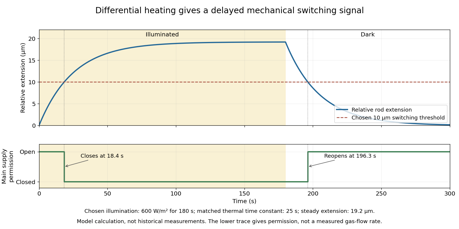
Take a stipulated pair of effective rods with common length $L$, linear thermal expansion coefficient ${\alpha }_L$, heat capacity $C$, projected illuminated area $A$, and thermal conductance $G$ to an environment at constant temperature $T_a$. One reference represents the symmetric polished-rod assembly. Write ${\theta }_b=T_b-T_a$ and ${\theta }_r=T_r-T_a$. Let their effective radiometric absorptances be $a_b>a_r$ for a fixed incident optical spectrum, and let $E(t)$ be the common irradiance. A spatially uniform, linear heat-balance model givesHere $G$ includes a linear approximation to the relevant losses; changing the surface treatment can also change those losses in a real device. We stipulate equal $C$ and $G$ to isolate the response to absorbed illumination, with thermal coupling from the burner neglected. Small, mechanically unconstrained extensions then give a differential displacementThe time constant $\tau$ describes thermal memory. A common imposed temperature shift cancels from the extension difference under the matched-coefficient assumptions; mismatched materials, geometry or thermal coupling can spoil that cancellation.

For a step from darkness to constant irradiance $E_0$, with initially equal rod temperatures, the first-order linear differential equation givesChoose $L=0.20\mathrm{m}$, ${\alpha }_L=20\times 10^{-6}{\mathrm{K}}^{-1}$, $A=0.0020{\mathrm{m}}^2$, $a_b=0.9$, $a_r=0.1$, $C=5.0\mathrm{J}{\mathrm{K}}^{-1}$, $G=0.20\mathrm{W}{\mathrm{K}}^{-1}$ and $E_0=600\mathrm{W}{\mathrm{m}}^{-2}$. The calculated difference of absorbed powers is $0.96\mathrm{W}$, givingFor an illustrative ideal valve that closes at $\delta =g=10\mu \mathrm{m}$, the closing time isThis threshold is crossed only when $0<g<{\delta }_{\infty }$. These are chosen model parameters, not a fit to a historical valve.

After illumination stops at $t=t_1$, the displacement decays as $\delta (t)=\delta (t_1)e^{-(t-t_1)/\tau }$. With $t_1=180\mathrm{s}$, the model reopens about $16.3\mathrm{s}$ later. Thus a sun valve responds to the thermal history of illumination; it does not read a clock or directly measure the beacon's brightness.

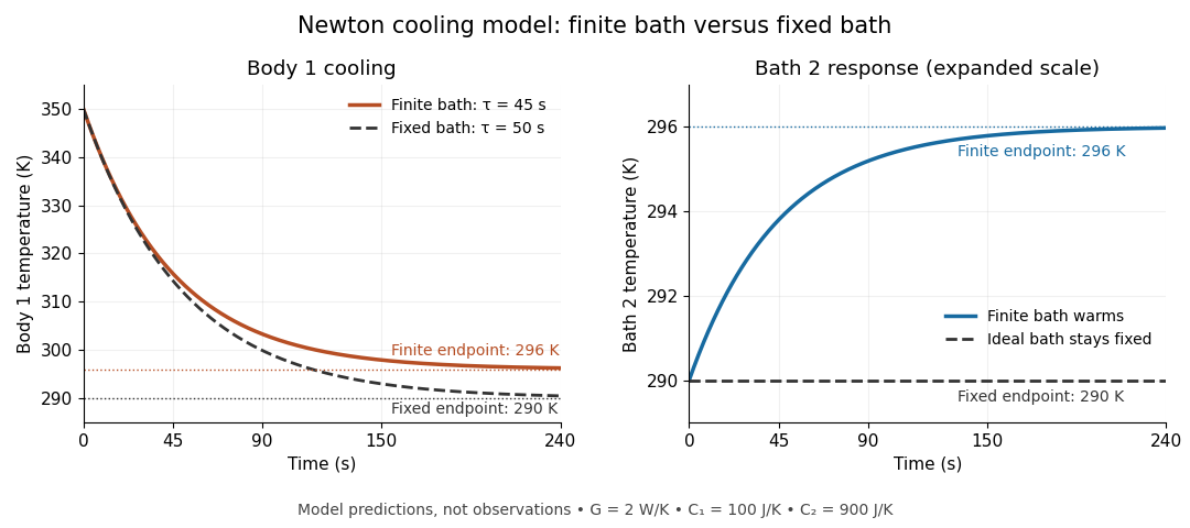
The equilibrium calculation determines where the two temperatures end, without determining how long they take. Stipulate a constant thermal conductance $G>0$ and the linear heat transfer law underlying Newton's law of cooling. With $Q$ positive from body 1 to bath 2, the ordinary differential equations areThe dot denotes a derivative with respect to time. This model assumes internal equilibration is fast compared with exchange between the bodies. Adding the two energy rates gives zero; subtracting the temperature rates givesThe temperature difference has exponential decay with time constant $\tau$. For the finite heat bath example and the stipulated $G=2\mathrm{W}{\mathrm{K}}^{-1}=2\mathrm{J}{\mathrm{s}}^{-1}{\mathrm{K}}^{-1}$, $\tau =45\mathrm{s}$, and solving the ordinary differential equations givesAt one time constant, $T_1\simeq 315.865\mathrm{K}$, $T_2\simeq 293.793\mathrm{K}$ and $Q\simeq 3413.451\mathrm{J}$. Equal temperatures are approached as a limit at infinite time. The finite bath causes the temperature difference to shrink faster than the fixed-bath model, because both bodies change temperature.

For an ideal heat bath with the same $G$, set $T_2=T_b=290\mathrm{K}$ rather than evolving its temperature. Newton's law of cooling then yieldsChanging $G$ changes these time constants, while the final temperature is fixed by the capacities and initial conditions. The dynamical model independently checks the Second law of thermodynamics:Its integral over the relaxation reproduces the endpoint entropy change. The useful separation is between capacity, which governs how much the bath temperature shifts, and thermal conductance, which governs the exchange rate. Neither alone establishes a reliable heat bath.

A controlled thermal link: high thermal conductance lets a cold stage equilibrate with a heat bath; low thermal conductance suppresses heat transfer during adiabatic demagnetization.

Three distinct effects spoil indefinite $T\propto B$ cooling: extra entropy outside the spin subsystem, additional magnetic energy scales, and irreversible heat or work input. They can be distinguished with a thermodynamic derivative. For a smooth equilibrium Helmholtz free energy obeying $dF=-SdT-mdB$, a Maxwell relation givesHere $C_B$ is the total heat capacity participating in the stage's thermal equilibrium. The ideal model has $(\partial m/\partial T{)}_B=-C_{B,\mathrm{mag}}/B$. If its spins share temperature with a field-independent lattice and load of combined heat capacity $C_{\mathrm{other}}>0$, thenThe positive slope still means cooling when $dB<0$, but its smaller magnitude gives less cooling per fractional field reduction. For example, a low-temperature Debye model gives a lattice entropy proportional to $T^3$. As that lattice entropy falls, the spins take up the released entropy; $x$ can no longer remain constant. A weak enough coupling to neglect its equilibrium interaction energy can still be strong enough to exchange heat on the sweep timescale.

Interactions between magnetic moments, including exchange interaction and the fields of neighboring magnetic dipole moments, introduce energy scales that do not vanish with the applied $B$. Once they compete with $k_{B}T$ or $\mu B$, the independent-site partition function fails. Correlations and possible magnetic ordering alter the available magnetic entropy and the cooling curve. Simply setting the external magnetic field to zero does not eliminate those interactions. Different refrigerants therefore need their own measured equilibrium properties; there is no universal final temperature from the applied-field ratio alone.

Finally, a real open heat switch has residual thermal conductance; supports, wires and radiation carry incoming heat. Field changes may also dissipate energy. Locally near thermal equilibrium, with incoming heat rate ${\dot{Q}}_{\mathrm{leak}}$ and internal entropy production rate ${\dot{S}}_{\mathrm{prod}}$, the stage balance becomesThis uses a common stage temperature; a non-equilibrated load requires separate balances. The sweep must allow spin-lattice relaxation while remaining fast enough to limit accumulated parasitic heat. At fixed $B$, the same balance explains warming and finite hold time. Useful refrigeration is the controlled absorption of a load's heat during that finite interval, followed by a renewed isothermal process of magnetization to export its entropy.

Low-temperature calorimetry measures a small sample's heat capacity by resolving a small temperature change after a known electrical energy input. The experimental challenge is that the support, heater and thermometer also warm up. Their calorimeter addenda must be removed before interpreting the sample's phonons or electronic heat capacity. The Debye T-cubed test turns the corrected response into a test of the low-temperature vibrational spectrum.

Manuel Brando's 2009 experiment used a sapphire platform suspended by four alloyed platinum wires from a copper ring fixed to a cryostat stage. Grease attached the sample; a chip heater and ruthenium-oxide resistance thermometer served platform PLS-2. A controller stabilized the bath; a lock-in amplifier supplied heating pulses and read the calibrated sensor. The steady rise calibrated thermal conductance as $G=P/\Delta T$. A separate $59.1\mathrm{mg}$, $99.99\%$ pure gold sample, compared with reference heat capacities, established the calorimeter addenda. Small pulses limited property variation; imperfect sample contact required a second relaxation time. The platform contribution rose below $1.5\mathrm{K}$, making simple extrapolation unsafe.^[ref]

For an original idealization, assume sample and platform share one temperature $T$, the bath remains at $T_b$, and both the total heat capacity and the weak-link thermal conductance $G$ are approximately constant across one small pulse. Ignore other heat transfer and any phase transition. The first law of thermodynamics becomesHere $C_s$ is sample heat capacity, $C_a$ is calorimeter addenda, $P$ is deposited electrical power from Joule heating, and $\tau$ is a time constant. This is the same balance as calorimeter heat-loss correction, used here with a deliberately weak cryogenic link and a separately subtracted platform. For a constant pulse $P_0$ beginning at bath temperature, then switched off at $t_h$,The cooling exponential decay determines $\tau$, while the heating plateau determines $G=P_0/(T_{\infty }-T_b)$. Together with calorimeter addenda, they give $C_s=G\tau -C_a$. Cooling alone determines a ratio, not an absolute heat capacity. With finite $t_h$, the observed end rise is smaller than the plateau; fit the full response or apply the displayed correction rather than identifying the two.

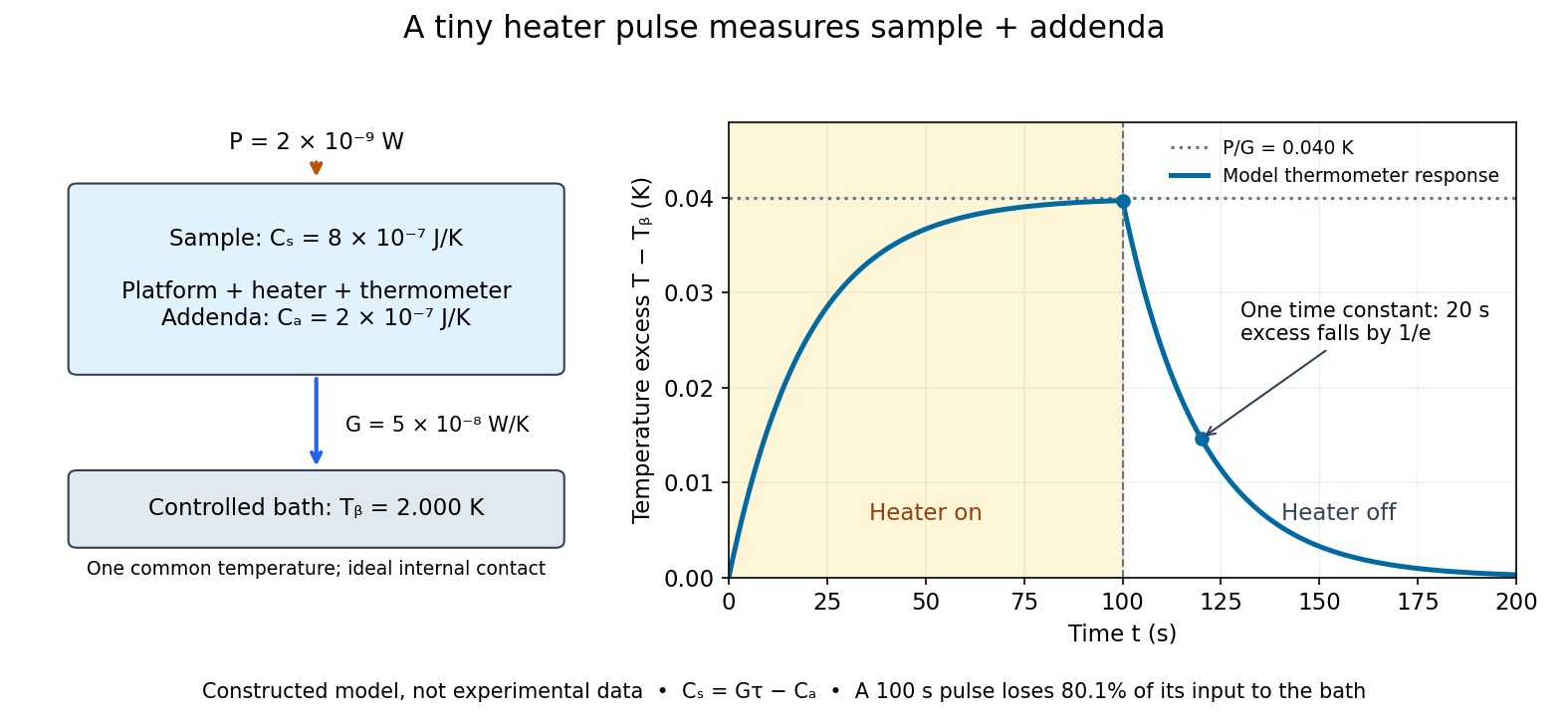
For the stipulated figure parameters, $G=5.00\times 10^{-8}\mathrm{W}{\mathrm{K}}^{-1}$, $\tau =20.0\mathrm{s}$, and $C_a=2.00\times 10^{-7}\mathrm{J}{\mathrm{K}}^{-1}$ give $C_s=8.00\times 10^{-7}\mathrm{J}{\mathrm{K}}^{-1}$. The asymptotic rise is $0.0400\mathrm{K}$, only $2\%$ of bath temperature. At $100\mathrm{s}$, the rise is $0.0397305\mathrm{K}$. Of $2.00\times 10^{-7}\mathrm{J}$ input, only $3.97305\times 10^{-8}\mathrm{J}$ remains stored: the other $1.60270\times 10^{-7}\mathrm{J}$ has flowed to the bath. Treating this long pulse as an isolated $Q/C$ experiment would overestimate total heat capacity by a factor of $5.034$.

Suppose independent standard uncertainties are $u(G)=0.05\times 10^{-8}\mathrm{W}{\mathrm{K}}^{-1}$, $u(\tau )=0.2\mathrm{s}$ and $u(C_a)=0.10\times 10^{-7}\mathrm{J}{\mathrm{K}}^{-1}$. First-order propagation of uncertainty givesThe uncertainty is one standard deviation under those assumptions, about $2.2\%$ of sample heat capacity. Shared thermometer calibration errors can correlate fitted $G$ and $\tau$; then their covariance contributes too. Smaller samples amplify the relative influence of calorimeter addenda. Proposed checks include varying pulse amplitude, repeating with a reference sample, checking sensor self-heating, and comparing single- and two-time-constant fits. A drifting bath, slow internal equilibration or a transition invalidates this simple reduction even if a cooling curve looks smooth.

Temperature changes affect measurements through several routes. Thermal expansion changes lengths and alignments; temperature-dependent resistance and refractive index change electrical and optical calibrations; temperature differences between dissimilar junctions generate Seebeck effect voltages. These slow environmental changes are distinct from unavoidable equilibrium thermal fluctuations and Johnson-Nyquist noise. A useful strategy identifies the coupling to the measured signal before choosing a remedy.

Reduce environmental coupling by enclosing the apparatus against drafts, using thermal insulation and radiation shields, isolating heat sources, and minimizing dissipated power. A vacuum enclosure suppresses convection but leaves thermal conduction and thermal radiation paths to control. A large heat capacity reduces rapid temperature excursions. In a simple thermal model with heat capacity $C_T$ and thermal conductance $G_T$ to a reservoir, the relaxation time is $C_T/G_T$, so adequate settling time is necessary after changing the apparatus. A temperature sensor close to the sensitive element and stable negative feedback heating or cooling can regulate its temperature; poorly placed sensors or excessive feedback gain can leave gradients or cause oscillations.

Electrical thermal noise has the classical low-frequency one-sided voltage power spectral densityfor a resistor measured over a flat bandwidth $B$ without significant loading. More generally replace $B$ by the effective noise bandwidth. Lower temperature or narrower bandwidth reduces the noise, and resistance choices must account for source loading and the amplifier's own voltage and current noise. A lock-in amplifier uses modulation and narrowband detection to reject much low-frequency drift and out-of-band noise, while thermal noise inside the accepted band remains. Temperature stabilization does not remove equilibrium fluctuations.

Use a matched reference or differential bridge to reject common environmental changes. Keep junctions isothermal and choose matched materials to reduce thermoelectric offsets. For a resistance measurement, reversing a small test current separates a stable offset from the wanted voltage:Reversal must be fast enough that the offset stays approximately fixed, with enough settling time and sufficiently little self-heating. Recording the sample temperature permits a measured calibration slope $dS/dT$ to correct a signal to a reference temperature; the correction's calibration and thermometer uncertainties must be propagated. Independent white noise fluctuations decrease under averaging, whereas correlated temperature drift may not decrease as the inverse square root of the number of readings. Temperature records and repeated reference measurements help distinguish the two.

Thermal conductance is the heat transfer rate divided by the driving temperature difference in a linear contact model. It is the reciprocal of thermal resistance, with units $\mathrm{W}{\mathrm{K}}^{-1}$; thus $\dot{Q}=G(T_1-T_2)$ for heat transferred from body 1 to body 2.

Thermoelectric cooling uses the Peltier effect to remove heat from a load using electrical work. A typical thermoelectric module connects many pairs of different semiconductors electrically in a series circuit and thermally in parallel between two faces. For an idealized pair with $S_p>S_n$, positive conventional current crosses n to p at the cold bridge and p to n at the hot return. With common bridge material and isothermal contacts, the intervening metal contributions telescope: the net pair coefficient is $S_p-S_n$. For $N$ identical pairs define the module Seebeck coefficient $\alpha =N(S_p-S_n)>0$.

Choose fixed face temperatures $T_h\ge T_c>0$, $\Delta T=T_h-T_c$, module electrical resistance $R>0$ and open-circuit thermal conductance $K>0$. All three module parameters $\alpha ,R,K$ are constants over the chosen operating range. Positive $I$ is the orientation absorbing Peltier effect heat at c. Define $Q_c$ as net heat extracted from the cold reservoir per unit time, $Q_h$ as net heat delivered to the hot reservoir per unit time, and $P_{\mathrm{in}}$ as electrical power entering the module. Despite the conventional letters $Q_c,Q_h$, both denote power in watts, not accumulated energy. Ferrotec gives the corresponding single-stage equations and distinguishes module performance from bypass leaks.^[ref]

A useful original model treats the thermopile absorber as one approximately uniform temperature $T_h(t)$ with heat capacity $C_{\mathrm{th}}$, connected to a fixed reference temperature $T_c$ by thermal conductance $G_{\mathrm{th}}$. Both parameters are positive constants here. Let $P_{\mathrm{abs}}(t)$ be an added absorbed power above the initial background. Linearize the outgoing heat transfer about that background. With $\Delta T=T_h-T_c$ measured from an initial state having $\Delta T=0$, conservation of energy gives the first-order linear differential equationThe left side is the rate of stored energy; the two terms on the right are added power and outgoing heat transfer. The effective thermal conductance can include several paths, rather than just heat conduction along the wires. The model assumes a stable reference, negligible electrical loading, a common absorber temperature, and changes small enough for constant parameters.

For a step from zero to constant $P_0$ at $t=0$, subtract the steady solution $\Delta T_{\infty }=P_0/G_{\mathrm{th}}$. The difference obeys exponential decay, so the initial condition fixesThe time constant has units $(\mathrm{J}{\mathrm{K}}^{-1})/(\mathrm{W}{\mathrm{K}}^{-1})=\mathrm{s}$. With the same constructed $N=20$ and $\alpha =40\mu \mathrm{V}{\mathrm{K}}^{-1}$, choose $C_{\mathrm{th}}=0.02\mathrm{J}{\mathrm{K}}^{-1}$, $G_{\mathrm{th}}=0.01\mathrm{W}{\mathrm{K}}^{-1}$ and $P_0=0.03\mathrm{W}$. ThenAt one time constant, the response is $1-e^{-1}\approx 0.632$ of its final value: $V_{\mathrm{oc}}(2\mathrm{s})\approx 1.52\mathrm{mV}$. Reaching $95\%$ requires $t=-\tau \ln (0.05)\approx 5.99\mathrm{s}$. A voltmeter read too soon therefore underestimates the steady signal even when its electrical calibration is perfect.

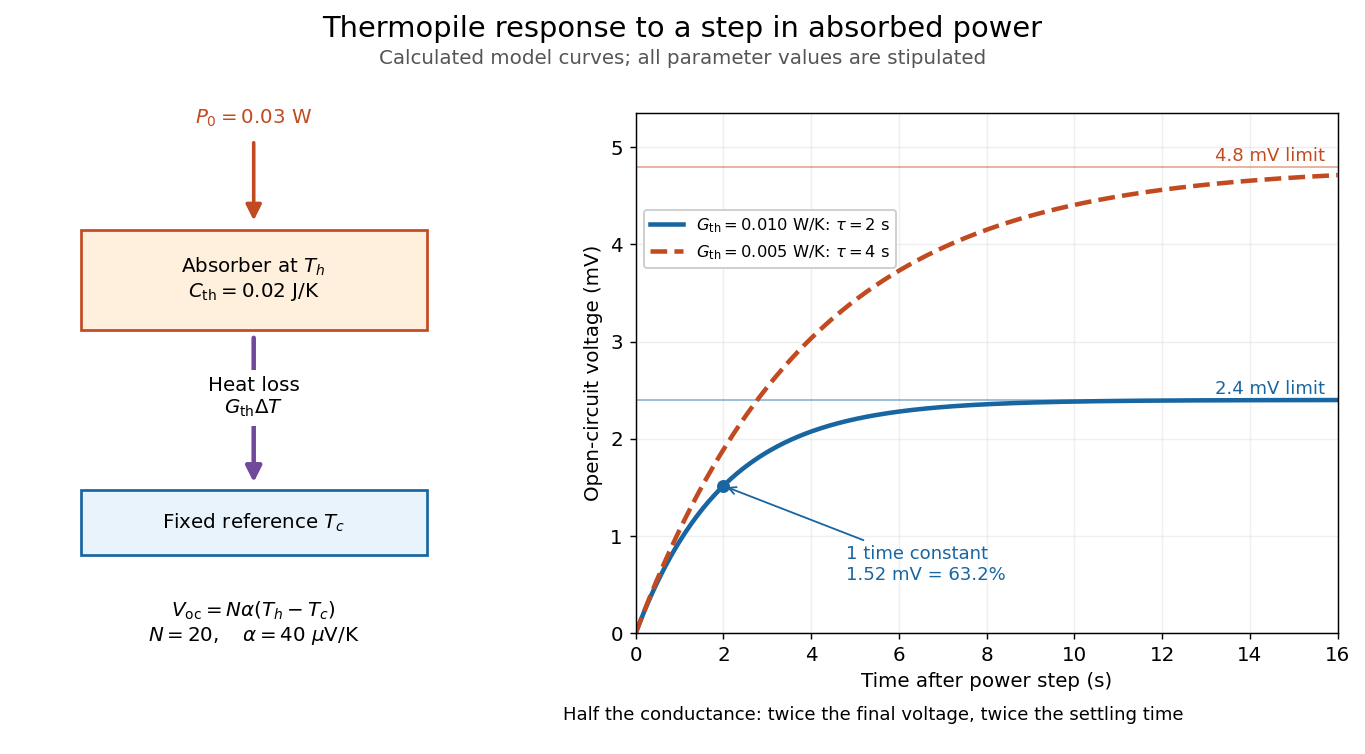
The steady ratio $V_{\infty }/P_0=N\alpha /G_{\mathrm{th}}$ is $0.080\mathrm{V}{\mathrm{W}}^{-1}$ in this constructed model. Halving thermal conductance doubles this ratio but also doubles the time constant if heat capacity stays fixed. Reducing heat capacity alone speeds the response without changing its steady value. Increasing $N$ gives a larger signal only at fixed individual temperature differences: adding legs can also change thermal conductance, heat capacity and electrical resistance. The algebra identifies coupled design choices, rather than predicting a particular manufactured detector.

A finite electrical resistance produces Thermal electrical noise. For nearly uniform absolute temperature $T$ and effective measurement signal bandwidth $B$, its root mean square open-circuit voltage isHere $k_{\mathrm{B}}$ is the Boltzmann constant. Thermal electrical noise in the sensing element is an important contribution, and the signal bandwidth enters its voltage variance.^[ref] If identical pairs have fixed electrical resistance $r$ and fixed $\Delta T$, then $R_{\mathrm{pile}}=Nr$: the signal grows as $N$ while this noise grows as $\sqrt{N}$. The resulting signal-to-noise ratio grows only as $\sqrt{N}$ under those assumptions. Reference temperature drift, environmental electromagnetic radiation, and meter noise remain separate limits; reducing signal bandwidth trades fast information for less integrated electrical noise.