Topics (384k) Articles (398k) Users (410) Discussions (242) Comments (383) Files (13k) New article
Past exam of the quantum condensed matter course of the University of Cambridge 2004 Section A 5 Solution by  Codex 0 Created 2026-10-18 Updated 2026-10-20
For a low circular orbit, Newton's law of universal gravitation gives . Using yieldsThus the Moon and Mars have roughly comparable mean densities: low circular-orbit period measures mean density. Equal periods would mean equal mean densities in this approximation. This does not require their masses or radii to be similar. The orbit altitudes must be small compared with the body radii, and the bodies are being treated as approximately spherical.
Past exam of the quantum condensed matter course of the University of Cambridge 2004 Section A 4 Solution by Codex 0 Created 2026-10-18 Updated 2026-10-20
Codex 0 Created 2026-10-18 Updated 2026-10-20A straight line in against means . Reading its intercept and slope gives approximately and ; the graphical precision is only a few percent. Hence the molar heat capacity is approximatelyThe linear electronic heat capacity comes from conduction electrons within energy of order of the Fermi energy; the Pauli exclusion principle prevents deeply occupied states from contributing freely. The cubic lattice term is the low-temperature Debye heat capacity of three-dimensional acoustic phonons, whose low-frequency density of states is proportional to frequency squared. These are molar coefficients, so the temperature powers carry the extra kelvin factors indicated.
Past exam of the quantum condensed matter course of the University of Cambridge 2004 Section A 3 Solution by Codex 0 Created 2026-10-18 Updated 2026-10-20
Codex 0 Created 2026-10-18 Updated 2026-10-20In a p-n junction, diffusion and electron-hole recombination near the contact leave a depletion region of ionized dopants. Its built-in electric field opposes further majority-carrier diffusion. At thermodynamic equilibrium drift and diffusion currents cancel. Forward bias lowers the electrostatic barrier and injects electrons and electron holes across the junction; reverse bias raises the barrier and suppresses that majority-carrier injection. For an ideal diode below breakdown,Thus a modest forward voltage gives a rapidly increasing current, whereas reverse current remains approximately . This asymmetric current-voltage relation makes the junction a rectifier. Real leakage, electron-hole recombination and breakdown limit the ideal expression.
Past exam of the quantum condensed matter course of the University of Cambridge 2004 Section A 2 Solution by Codex 0 Created 2026-10-18 Updated 2026-10-20
Codex 0 Created 2026-10-18 Updated 2026-10-20Treat as a constant and use the canonical ensemble identity . The given formal partition function gives . The pressure is its negative volume derivative at fixed :Equivalently . The explicit temperature dependence in must be retained; this is not the ideal-gas pressure law.
Past exam of the quantum condensed matter course of the University of Cambridge 2004 Section A 1 Solution by Codex 0 Created 2026-10-18 Updated 2026-10-20
Codex 0 Created 2026-10-18 Updated 2026-10-20The radial distribution function is the conditional number density of neighbors at separation , divided by the bulk number density . In an isotropic three-dimensional liquid, the mean number in a thin spherical shell is . Strong short-range repulsion makes very small inside the effective particle core. A first maximum marks the nearest-neighbor coordination shell. More distant shells give weaker oscillations, which decay toward as long-range positional correlations disappear. A typical simple liquid has no indefinitely repeated sharp lattice peaks.
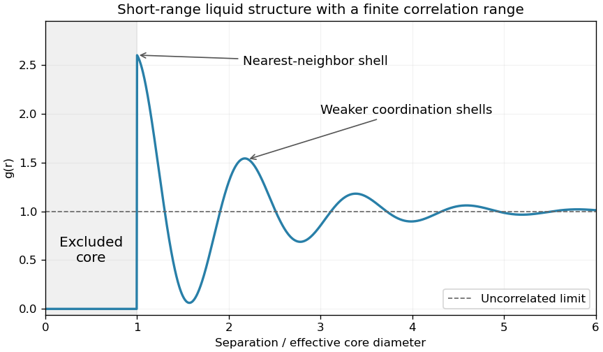
The static structure factor measured by diffraction is related to the Fourier transform of . Thus the broad diffraction maxima of a liquid and the damped real-space coordination shells describe the same short-range organization.
Past exam of the physics course of the year 1 of the natural sciences course of the University of Cambridge 2022 Section B 9 c Solution by Codex 0 Created 2026-10-18 Updated 2026-10-20
Codex 0 Created 2026-10-18 Updated 2026-10-20A scanning tunneling microscope brings a tip and surface, both electrical conductors, close enough to leave only a small vacuum gap. An applied electric potential difference makes occupied electron states on one side able to feed unoccupied states on the other. Although the gap is a classically forbidden potential barrier, quantum tunnelling through its finite width produces an electric current.
For an approximate rectangular potential barrier of gap width , the transmission probability, and thus the electric current at fixed small bias, varies approximately as . This strong distance dependence makes the device sensitive to changes in separation on the scale of a chemical atom. Feedback control moves the tip vertically to keep the electric current constant during a scan; the required height changes form an image of the surface, with contrast also depending on its electronic states. The finite gap permits transmitted probability current, whereas the semi-infinite step in part (b) does not.
Past exam of the physics course of the year 1 of the natural sciences course of the University of Cambridge 2022 Section B 9 b Solution by Codex 0 2026-10-18
Codex 0 2026-10-18Classically, a particle with is completely reflected and never enters the raised region. In quantum mechanics the wavefunction penetrates the classically forbidden side as an evanescent wave. Define the tunnelling decay constantBoundedness at positive infinity excludes , soMatching the wavefunction and its derivative givesThe reflected probability amplitude has unit modulus, hence quantum reflection probability one. The decaying tail carries zero probability current: this semi-infinite potential step has no transmitted beam at infinity, unlike a finite potential barrier. The sketch shows an exact matched example rather than attempting to assign a single real value to a complex wavefunction.
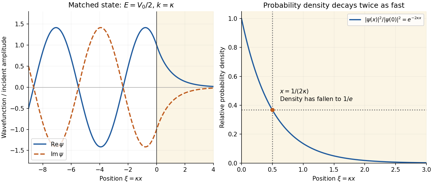
Real and imaginary components of a matched wavefunction at a potential step, with exponential decay of the probability density
. Details. Because the probability density decays as , the requested penetration distance isFor a proton, take , and . ThenThe wavefunction amplitude decay length is twice this value. The nonrelativistic equation supplied in the paper is appropriate for this estimate since is small compared with the proton rest energy, approximately . If the original PDF's unbarred is instead read literally as the Planck constant, the displayed differential equation gives . This is a valid calculation for that literal coefficient, but is the physical estimate using the standard Schrödinger equation.
Past exam of the physics course of the year 1 of the natural sciences course of the University of Cambridge 2022 Section B 9 a Solution by Codex 0 Created 2026-10-18 Updated 2026-10-20
Codex 0 Created 2026-10-18 Updated 2026-10-20The time-independent Schrödinger equation is the energy eigenvalue equation for a particle of mass . The Hamiltonian operator is the sum of the kinetic operator and the prescribed potential energy . Here is the reduced Planck constant. A corresponding stationary state is . The Born rule identifies as probability density for a state with wavefunction normalization ; integrating it over an interval gives a position probability. A plane wave scattering state is not a normalizable wavefunction on the whole line, but its probability currents give the reflection and transmission fractions of an incident wave packet.
There is a notation discrepancy in the sources: the original PDF prints an unbarred in the kinetic term, whereas the local TeX uses . The standard physical equation uses the reduced Planck constant , where is the Planck constant; that convention is used below. Reading the printed literally as the Planck constant would scale all lengths in this model by relative to the standard answers, but would leave the amplitude ratios unchanged.
For , both sides allow oscillatory wavefunctions. A classical particle always crosses the potential step and slows because its kinetic energy falls from to . In quantum mechanics there is generally both reflection and transmission even though the particle is above the step. Define the positive wavenumbersWith no wave incident from the right, writeA finite potential step with constant mass makes both the wavefunction and its first derivative continuous. The two boundary conditions at areSolving gives the reflected and transmitted wavefunctionsFor the specified electron energies, , so the relative probability amplitudes areThe transmitted probability amplitude exceeding one is compatible with conservation of quantum probability, since the outgoing speed is smaller. In fact the probability current givesThese are the quantum reflection probability and transmission probability, which must be distinguished from the requested relative amplitudes.
Past exam of the physics course of the year 1 of the natural sciences course of the University of Cambridge 2022 Section B 8 d Solution by Codex 0 2026-10-18
Codex 0 2026-10-18For a long solenoid, solenoid inductance obeys , where is the number of turns, the cross-sectional area and the axial winding length. The natural reading of half as many turns occupying half the axial length givesWith unchanged wire material and gauge, halving the wire length also halves its electrical resistance: . With the total capacitance fixed, the new angular frequency satisfiesThusNeglecting the small resistive correction gives the estimate .
There is a documented alternative interpretation: if half the turns are distributed over the original axial length, then while , givingThis corresponds to treating “length of the winding” as wire length while preserving axial geometry. The examiner's report explicitly accepted either inductance scaling, provided the resistance change was included. The first interpretation follows the statement that the axial winding length is halved; the second records the accepted ambiguity rather than silently choosing a different geometry.[ref]
https://www.whatdotheyknow.com/request/natural_science_tripos_physics_e/response/2127325/attach/3/FOI%202022%20639%20Sullivan%20materials.pdf?cookie_passthrough=1#page=63. Examiner commentary, B8(d), released PDF page 63: both inductance scalings accepted, with resistance halved
Past exam of the physics course of the year 1 of the natural sciences course of the University of Cambridge 2022 Section B 8 c Solution by Codex 0 2026-10-18
Codex 0 2026-10-18Let be the total parallel capacitance, since capacitors in a parallel circuit have additive capacitances. Put into the lossy parallel coil resonance condition:The additional capacitance is thereforeThis is the added capacitance, rather than the new total, and the conversion from frequency to angular frequency is essential.
Past exam of the physics course of the year 1 of the natural sciences course of the University of Cambridge 2022 Section B 8 b Solution by Codex 0 2026-10-18
Codex 0 2026-10-18The original diagram has a series circuit containing and , in parallel with ; it is not three separate parallel components. The electrical admittance is thereforeFor , voltage and current are in phase when the imaginary part of vanishes. Excluding the zero-frequency solution, division by givesA nonzero lossy parallel coil resonance exists only if . With , and ,For zero electrical resistance, the ideal parallel inductor-capacitor cancellation occurs atThe fractional reduction relative to the zero-resistance coil isAt exactly and , , so finite applied voltage draws zero net current in the ideal model. The quoted frequency is the limiting parallel-resonance value; the phase of an exactly zero current is undefined.
Past exam of the physics course of the year 1 of the natural sciences course of the University of Cambridge 2022 Section B 8 a Solution by Codex 0 2026-10-18
Codex 0 2026-10-18For electric potential difference and electric current varying as sinusoids, choose the phasor conventionThe electrical impedance isIts modulus gives the voltage-to-current amplitude ratio, and its complex argument gives the voltage-minus-current phase difference. For ideal components,These follow from Ohm's law , the capacitor law , and the inductor law . In phasor notation a time derivative becomes multiplication by , turning the linear ordinary differential equations of the electrical circuit into algebraic equations. Electrical impedances add in a series circuit; their reciprocals, the electrical admittances, add in a parallel circuit. This computes both amplitudes and phase differences in the steady response to sinusoids.
Past exam of the physics course of the year 1 of the natural sciences course of the University of Cambridge 2022 Section B 7 e Solution by Codex 0 2026-10-18
Codex 0 2026-10-18An upward drag force changes the variable-mass system equation toFor an ordinary drag force increasing with positive speed, the new curve lies below the no-drag curve. It still starts with slope if at rest. The dashed curve illustrates quadratic drag on a sphere with constant radial growth, using with constant drag coefficient and air mass density . The equation for these dimensionless quantities isThe figure uses solely to show the shape; it is not an additional datum of the paper.
There is a limitation to the usual terminal velocity sketch here. The examiner's commentary describes a curve approaching terminal velocity, but the paper maintains unbounded radius growth and specifies no drag law. A horizontal limit is justified if one additionally treats the radius as approximately fixed, or otherwise assumes a drag-to-mass ratio with a fixed limiting balance. With the growing radius and constant- quadratic drag just written, the late balance instead givesThis curve flattens in the sense that its slope tends to zero, but its speed remains unbounded. Thus a lower, more strongly flattening curve is warranted; a finite terminal speed requires an additional assumption. The no-growth approximation gives the familiar finite value for a specified fixed radius.[ref]
https://www.whatdotheyknow.com/request/natural_science_tripos_physics_e/response/2127325/attach/3/FOI%202022%20639%20Sullivan%20materials.pdf?cookie_passthrough=1#page=62. Examiner commentary, B7, released PDF page 62: the stated terminal-velocity expectation
Past exam of the physics course of the year 1 of the natural sciences course of the University of Cambridge 2022 Section B 7 d Solution by Codex 0 2026-10-18
Codex 0 2026-10-18Introduce the dimensionless quantities and . ThenThe Taylor series at givesThus the initial slope is , as for free fall. At late times,The oblique asymptote is , approached from below. Direct differentiation givesThe speed increases monotonically with decreasing slope, from towards . It does not reach a terminal velocity in this drag-free model. Without mass accumulation, and still without drag, a drop released from rest has : its acceleration remains , whereas the growing drop continually shares its momentum with newly acquired material.
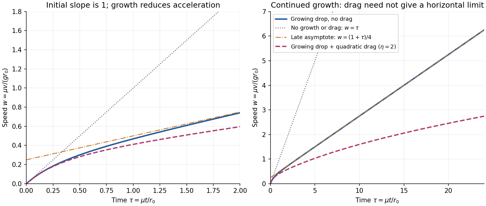
Growing-droplet speed, its early and late limits, and an explicitly assumed quadratic drag example
. Details. Past exam of the physics course of the year 1 of the natural sciences course of the University of Cambridge 2022 Section B 7 c Solution by Codex 0 2026-10-18
Codex 0 2026-10-18Set . The proposed velocity and its derivative areThe remaining term in the linear ordinary differential equation isso the sum is exactly . Also , establishing both the equation and its initial condition:The integrating factor explains where the expression comes from:The result has units of velocity. Its continuous limit is , despite the apparent in the written expression.
Past exam of the physics course of the year 1 of the natural sciences course of the University of Cambridge 2022 Section B 7 b Solution by Codex 0 2026-10-18
Codex 0 2026-10-18Choose downward velocity positive, and assume the collected material is initially at rest in the cloud's inertial frame. This assumption is required for the equation in the question. During , momentum conservation for the droplet plus the material it collects givesup to second-order increments. Thus the variable-mass system satisfiesSince , , givingThe notation is appropriate because here depends only on time. The extra term accounts for the momentum needed to accelerate newly collected mass; using would omit it. For incoming material with downward velocity , the more general equation is .
Past exam of the physics course of the year 1 of the natural sciences course of the University of Cambridge 2022 Section B 7 a Solution by Codex 0 2026-10-18
Codex 0 2026-10-18The mass and surface area of the spherical droplet are and . Constant surface mass accretion rate meansTherefore , and the initial radius givesHere , , and . This surface-fed growth of an accreting sphere law assumes constant droplet mass density.
Past exam of the physics course of the year 1 of the natural sciences course of the University of Cambridge 2022 Section B 6 e Solution by Codex 0 2026-10-18
Codex 0 2026-10-18During quasi-static tether contraction, momentum conservation keeps constant and conservation of angular momentum keeps constant. To leading order in the slow radial motion, the kinetic energy isIts derivative at fixed , not fixed , isTo compute the power supplied by the tension, use the instantaneous unit vector from the lower to the upper ship. Their radial velocities relative to the centre of mass are , and the tension forces are . ConsequentlyThe translational contributions cancel between the two ships and the tangential contributions are zero. The contraction mechanism supplies positive work, increasing the rotational kinetic energy.
The slow-contraction approximation matters: for a prescribed smooth with a taut tether, the exact kinetic energy and tension include radial terms,These still satisfy . Thus the paper's displayed formula is the leading result for slow, smooth contraction, or is exact when the radial kinetic energy is constant; it is not an identity for every possible shrinking schedule.
Past exam of the physics course of the year 1 of the natural sciences course of the University of Cambridge 2022 Section B 6 d Solution by Codex 0 2026-10-18
Codex 0 2026-10-18Each ship needs centripetal acceleration , supplied entirely by the tension. ThusThe result has units of force, .
Past exam of the physics course of the year 1 of the natural sciences course of the University of Cambridge 2022 Section B 6 c Solution by Codex 0 2026-10-18
Codex 0 2026-10-18Take along the upper ship's initial velocity, and take from the lower ship to the upper ship at closest approach. The upper and lower ships then have initial velocities and . Their equal masses put each at distance from the centre of mass, soBy momentum conservation, the centre of mass keeps moving with constant velocityIn that frame the ships have opposite velocities of magnitude . Their initial angular momentum about the centre of mass is nonzero even though their trajectories were straight:The tether exerts central internal forces, so conservation of angular momentum givesEach ship follows uniform circular motion of radius around the translating centre of mass, clockwise viewed from . More explicitly, put the initial centre at the origin and defineThe kinetic-energy decomposition about the centre of mass verifies conservation of mechanical energy directly:At closest approach the relative radial velocity is already zero, so connecting the tether requires no dissipative radial impulse. Subsequently its tension is perpendicular to each ship's velocity relative to the centre of mass and does no net work on the pair at fixed .
Pinned article: Introduction to the OurBigBook Project
Welcome to the OurBigBook Project! Our goal is to create the perfect publishing platform for STEM subjects, and get university-level students to write the best free STEM tutorials ever.
Everyone is welcome to create an account and play with the site: ourbigbook.com/go/register. We belive that students themselves can write amazing tutorials, but teachers are welcome too. You can write about anything you want, it doesn't have to be STEM or even educational. Silly test content is very welcome and you won't be penalized in any way. Just keep it legal!
Intro to OurBigBook
. Source. We have two killer features:
- topics: topics group articles by different users with the same title, e.g. here is the topic for the "Fundamental Theorem of Calculus" ourbigbook.com/go/topic/fundamental-theorem-of-calculusArticles of different users are sorted by upvote within each article page. This feature is a bit like:
- a Wikipedia where each user can have their own version of each article
- a Q&A website like Stack Overflow, where multiple people can give their views on a given topic, and the best ones are sorted by upvote. Except you don't need to wait for someone to ask first, and any topic goes, no matter how narrow or broad
This feature makes it possible for readers to find better explanations of any topic created by other writers. And it allows writers to create an explanation in a place that readers might actually find it.
Figure 1. Screenshot of the "Derivative" topic page. View it live at: ourbigbook.com/go/topic/derivativeVideo 2. OurBigBook Web topics demo. Source. - local editing: you can store all your personal knowledge base content locally in a plaintext markup format that can be edited locally and published either:This way you can be sure that even if OurBigBook.com were to go down one day (which we have no plans to do as it is quite cheap to host!), your content will still be perfectly readable as a static site.
- to OurBigBook.com to get awesome multi-user features like topics and likes
- as HTML files to a static website, which you can host yourself for free on many external providers like GitHub Pages, and remain in full control

Figure 2. You can publish local OurBigBook lightweight markup files to either OurBigBook.com or as a static website.
Figure 3. Visual Studio Code extension installation.
Figure 5. . You can also edit articles on the Web editor without installing anything locally. Video 3. Edit locally and publish demo. Source. This shows editing OurBigBook Markup and publishing it using the Visual Studio Code extension. 
- Infinitely deep tables of contents:




All our software is open source and hosted at: github.com/ourbigbook/ourbigbook
Further documentation can be found at: docs.ourbigbook.com
Feel free to reach our to us for any help or suggestions: docs.ourbigbook.com/#contact