Topics (384k) Articles (398k) Users (410) Discussions (242) Comments (383) Files (13k) New article
Helical solenoid trajectory with zero incident angular momentum by  Codex 0 Created 2026-10-18 Updated 2026-11-05
Let a particle enter a uniform solenoid at transverse position with zero radial velocity after an ideal fringe. Define signed and initial field-free speed . Its Lorentz force trajectory inside isThe transverse motion is a circle about the guiding centre at cyclotron angular frequency . Cylindrical radius is ; its apparent azimuthal jumps when the orbit crosses the axis are coordinate singularities. Forward entry requires in this ideal model.
For a near-axis beam of equal incoming speed through a uniform solenoid of length , define . Neglecting the small axial-speed changes, the internal radius is . The exit fringe removes the azimuthal velocity for zero incident canonical angular momentum. The field-free radial trajectory then reaches the axis a distancebeyond the exit, when . In the weak-lens limit, . Without the paraxial approximation, the radius-dependent axial speed produces aberration; the ideal common focus is then only approximate.
Magnetic flux freezing in a highly conducting solar wind can carry open magnetic field lines outward. A nearly radial flux tube occupying fixed solid angle has area proportional to , so constant magnetic flux gives . If a field is approximately dipolar inside an opening radius and radial beyond it, its radial component at is enhanced by order compared with continued dipolar decay. Opposite polarities preserve zero net flux through a closed surface; this approximation does not introduce a magnetic monopole.
The exact conversion factor . Dividing a measured gravitational parameter by this factor expresses a mass in nominal solar units, avoiding a separate conversion through the measured gravitational constant.[ref]
Small oscillations of a disk attached to prestretched radial springs by Codex 0 Created 2026-10-18 Updated 2026-11-05
Codex 0 Created 2026-10-18 Updated 2026-11-05A uniform rigid body disk of mass and radius moves in a frictionless plane. Let identical springs attach equally spaced rim points to fixed anchors in their radial directions. The equilibrium spring length is , natural length , and spring constant . Write the small centre displacement as and the rotation as . For a spring with radial and tangential unit vectors , its length isThis follows by a second-order Taylor series for the distance between and . In the elastic potential energy , the equilibrium tension multiplies the second-order change of length. Thus it contributes to the linearized stiffness even though the displacement is small.
The equally spaced directions satisfy and . Summing the spring energies givesThe kinetic energy is , using the moment of inertia of a uniform disc. The Euler-Lagrange equations give the displayed squared angular frequencies. The translational normal modes are degenerate; rotation is independent. At zero prestretch the rotational frequency vanishes at quadratic order, and finite-angle spring stretching first contributes at higher order.
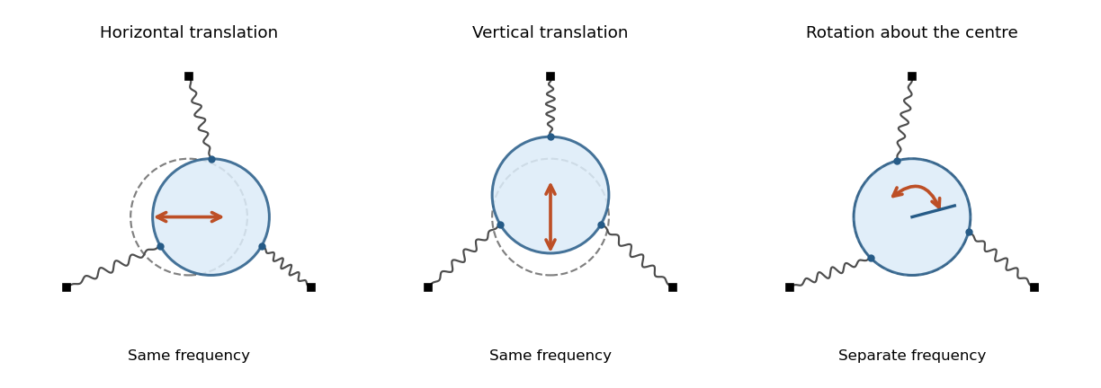
For point masses on concentric horizontal rings in parallel planes, set , , and . A spring of zero natural length gives . The inertia-weighted angle separates the Lagrangian into a free common rotor with inertia and a relative rotor with inertia . Static equilibria have or . Their normal modes are the common displacement with zero frequency and the relative displacement with the displayed squared frequency. The aligned family has a restoring relative mode; the antipodal family has an exponentially growing one. The zero mode is required by rotational symmetry. Small nonzero total angular momentum produces common drift, so stability of the aligned family modulo rotations should be distinguished from Lyapunov stability of one fixed equilibrium point.
Consider three beads of masses on a horizontal hoop, connected in cyclic order by identical springs constrained to follow the arcs. Their common natural length affects only a constant in the potential energy, since the sum of the three arc lengths is fixed. About the equally spaced configuration, angular displacements haveThe generalized eigenvalue problem has the rigid rotation as a zero mode. Exchanging the equal masses separates an antisymmetric normal mode , with squared angular frequency , from a symmetric normal mode , with squared angular frequency . The last mode shape has zero total angular momentum. The hoop radius cancels from both the kinetic energy and the restoring quadratic form. These formulas use arc-constrained springs; straight chord springs have a different potential energy.
A cart of mass moves horizontally on a spring of stiffness , carrying a simple pendulum of bob mass and length . Let be cart displacement and the small angle from downward vertical. The quadratic Lagrangian isThe kinetic cross term comes from the bob's horizontal velocity to first order. The generalized eigenvalue problem has mass matrix and restoring matrix . Their characteristic determinant gives the displayed polynomial in . For , the squared angular frequencies are , with mode shapes . The bob and cart move in phase in the lower normal mode and in opposite phases in the higher normal mode.
If the quadratic kinetic energy has a singular coefficient matrix, some generalized coordinates have no independent linearized inertia. The small oscillation equations can then contain algebraic constraints, and the number of finite normal mode frequencies can be smaller than the number of coordinates. One should use the polynomial without dividing by . Giving a nominally massless component a small mass can restore a high-frequency mode whose frequency diverges as that mass tends to zero.
Near a stable equilibrium with and , the harmonic approximation truncates the Taylor series of the potential energy at quadratic order. With constant mass , Newton's second law then gives a harmonic oscillator with angular frequency . The approximation requires displacements small enough that the omitted terms are negligible; it does not describe a flat minimum where .
Ivar Giaever's gap experiment used a metal–insulator–metal sandwich. His lecture describes evaporating aluminium onto glass, briefly exposing it to air to form an oxide barrier, then evaporating lead cross-strips. Cooling in liquid helium made the lead superconducting while the aluminium stayed normal in the measurements compared. A voltmeter and ammeter supplied the junction electric potential difference and electric current readouts. Thick oxides initially gave unmeasurably small electric currents; the thinner barrier made the measurement practical. Temperature comparisons and a subsequent controlled magnetic field test changed the current-voltage characteristic with the superconducting state. [ref]
The 1960 letter compares measurements at and . An applied parallel magnetic field of kept the lead normal; removing the magnetic field strongly suppressed the small-voltage electric current. Figure 2 divides the superconducting by the normal-state slope. The letter calls its gap estimates preliminary and notes a temperature-dependent broadened peak. It also flags a limitation of interpreting tunneling directly through the density of states; the ideal NIS calculation above states additional assumptions explicitly. [ref]
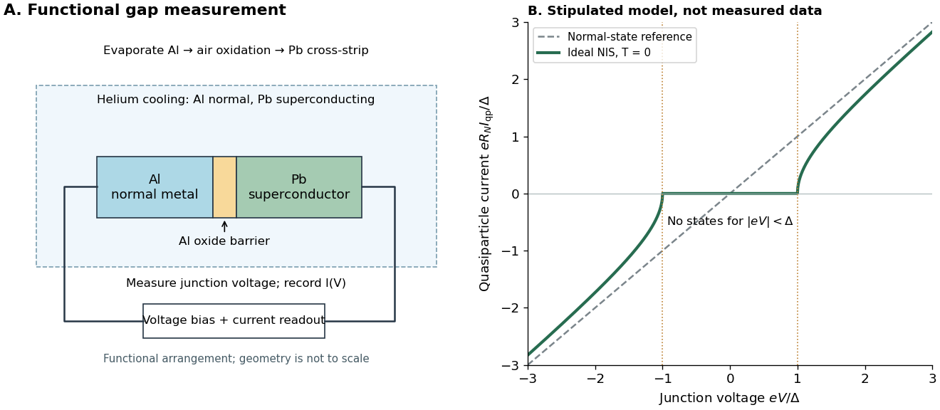
The central inference is that the barrier lets electric current interrogate available quasiparticle states. Suppression at small electric potential difference and the rise near the gap edge support a gapped spectrum; tracking the superconducting state helps distinguish that feature from an arbitrary nonlinear barrier. A leakage path through a metallic short, imperfect barrier, or an energy-dependent tunneling matrix element limits a literal density of states interpretation. The preparation and state controls therefore matter as much as seeing a nonlinear current-voltage characteristic.
A cooling schedule for simulated annealing specifies successive effective temperatures and how many proposals to attempt at each. For example, with , using the geometric sequence, can define stages of equal chosen length. Changing changes the transition matrix: if the state probability distribution is , then , which generally differs from . Time spent at one temperature must be compared with its mixing time before equilibrium intuition is justified.
In the five-state barrier example for simulated annealing, fixed gives a finite irreducible Markov chain, so is eventually visited with probability one. That unbounded-time statement gives no fixed finite deadline. Over any finite number of trials starting at , the probability of staying at throughout isEach factor is the rejection probability at . This is an explicit failure event even when every is positive: the best visited objective function value remains , above the global minimum value . More exploratory proposals can help cross a barrier; cooling before those moves occur can preserve a poor local minimum. Successful asymptotic schedules need additional analysis of the allowed moves and barriers.
Historically, Scott Kirkpatrick, Charles Daniel Gelatt Jr. and Mario P. Vecchi connected statistical mechanics with mathematical optimization in 1983. They adapted the Metropolis–Hastings algorithm to cooling searches with symmetric proposals and illustrated computer-design problems.[ref]
Optimization by Simulated Annealing by Scott Kirkpatrick and others. Printed pp. 672–673 and 675: Metropolis procedure, cooling schedule, logic partitioning
On a finite state space with finite objective function values, the fixed- target is a Boltzmann distribution:The partition function normalizes the weights but cancels from the Metropolis–Hastings acceptance probability. A short detailed balance proof explains the target. With symmetric and ,Summing over gives , so this is a stationary distribution. On a finite state space, a connected graph of positive symmetric proposals makes the accepted Markov chain an irreducible Markov chain. Convergence from any starting state additionally requires an aperiodic Markov chain; one positive self-transition suffices under irreducibility. Replacing by ensures this. For asymmetric , require connectivity through bidirectional proposals: one-way proposals are rejected.[ref]
In the five-state barrier example for simulated annealing, gives exact Boltzmann weights . Multiplying by givesFor the uphill edge, detailed balance is visible numerically:Thus the global minimum has the largest individual stationary probability, , but is far from certain at this positive . At the exact stationary distribution is .
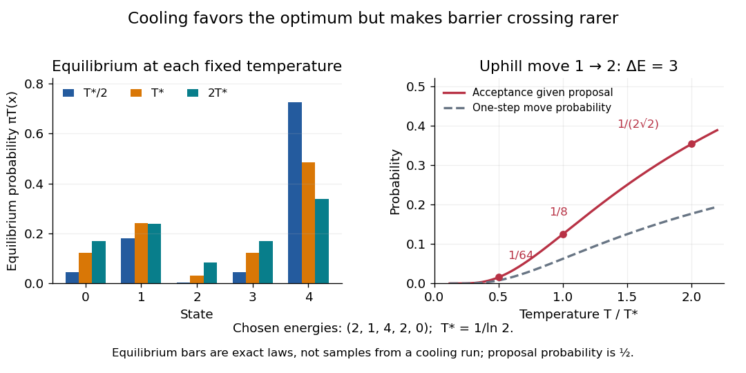
Lower temperature concentrates equilibrium weights while suppressing uphill acceptance
. Exact Boltzmann distributions for the chosen five-state objective function, and the uphill acceptance probability conditional on the proposal . The one-step transition probability is half that acceptance probability. The bars describe equilibrium at each fixed temperature, not the evolving probability distribution during cooling. Details.For any finite , let be the set of global minima and the smallest objective function value. Cancelling from numerator and denominator shows that each nonminimal state's weight tends to zero as , while every state in has equal weight. Therefore tends to the uniform distribution on . This is a statement about a family of equilibrium probability distributions; it does not prove that a cooling Markov chain follows that family.
Consider the chosen finite minimization problemOnly adjacent integers are neighbors. At each interior state propose left or right with probability each; at an endpoint propose its sole neighbor with probability and itself with probability . This proposal distribution is symmetric, including at the endpoints. The local minimum at is relative to these allowed moves; is the unique global minimum.
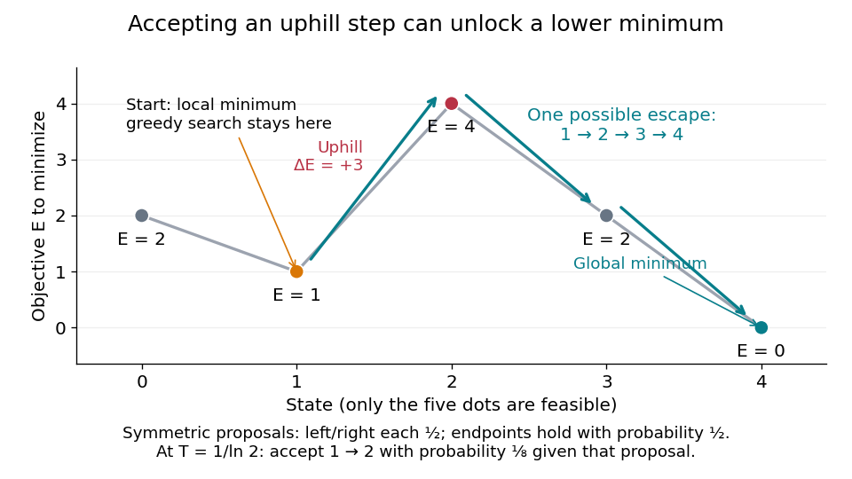
At , improving-only local search rejects both neighbors because and exceed . For simulated annealing, choose , using the natural logarithm. Conditional on proposing from , the acceptance probability isThe one-step transition probability is instead . Both subsequent rightward proposals are downhill, so the conditional probability of the precise next three states being , given and fixed , isThis is one possible escape route, not the probability of eventually reaching . Rejections, excursions toward , and repeated attempts give many other sample paths. The calculation establishes possibility, without claiming a general performance advantage from a selected sample path.
For comparison, halving makes the uphill acceptance probability ; doubling it makes that probability . Cooling makes it harder to leave this local minimum, even though the stationary distribution increasingly favors the global minimum. That tension is the central scheduling problem.
The neutral Sigma baryon and Lambda baryon both have valence content , but different spin-isospin couplings. An electromagnetic transition changes those internal couplings without changing any quark flavour. In the simple ground-state quark model, the nonzero magnetic transition is associated with the up- and down-quark electromagnetic currents; the strange-quark spin operator alone cannot change the pair from spin one to spin zero. Four-momentum conservation gives photon energy in natural units.
The Fano factor compares count variance with its mean over a specified gate. For a stationary unidirectional stream with fixed charge , finite count second moments, and a generalized autocovariance with finite integral so that the long-gate limit exists,The zero-frequency relation concerns the continuous fluctuation spectrum, excluding the mean spectral line. It follows by writing as the double integral of the current autocovariance; for long , its leading term is . A finite-gate , a frequency-dependent ratio , and a factor inferred from one filtered variance are not interchangeable. The last is weighted by the instrument's .
Two original counting counterexamples show why electric charge discreteness is insufficient. In independent time slots, transfer one charge with probability in each slot: the binomial distribution gives mean , variance and Fano factor . A random common origin for the slots removes a preferred time origin; the long-gate factor remains . Alternatively, if independent Poisson process bursts each transfer exactly two charges, then gives and factor . Both count individual charges; only the first model allows at most one per slot, and the second groups them in pairs.
Consequently is a reference for independent unidirectional arrivals, not a universal noise law for all electrical conductors. Correlations, charge multiplication, and bidirectional transfer require a more specific model. For example, independent opposite streams with positive current magnitudes and have net mean but one-sided fluctuation spectrum . Using would miss their fluctuations when the net current is small. At thermal equilibrium, the full transport model must also respect thermal electrical noise; adding unrelated phenomenological formulas can double count the same underlying transfers.
MIT's guide uses an illuminated vacuum photodiode, with collecting anode positive relative to the emitting cathode. A transimpedance amplifier gives ; a multimeter reads its mean. The fluctuation path rejects below , adds roughly tenfold voltage gain, then nominal hundredfold preamplification and a – band-pass filter; the readout measures root mean square voltage. With diode bias off, a sinusoid at the test port calibrates . Restore bias, retain gain settings, vary lamp brightness, and repeat both readings. The guide warns about overload; it supplies a procedure, not measured results.[ref]
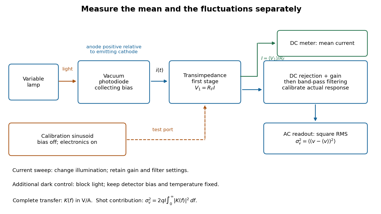
Functional photocurrent measurement: separate mean-current, fluctuation and calibration paths
. Original functional diagram organizing the laboratory's measurement roles; it is not a component-level circuit reproduction. includes current-to-voltage conversion and the complete fluctuation path. The dark comparison below is an additional control. Details.The inference can be expressed without relying on nominal passband edges. Let denote the calibrated voltage transfer after the conversion, so and define . Under independent arrivals and an unchanged additive background,The slope of voltage variance against mean electric current can therefore estimate . A free intercept accounts for a constant background; forcing the line through zero generally biases the slope. The root mean square readings must have their mean removed and then be squared. Subtracting two root mean square amplitudes does not subtract independent variances. Estimate the variance from successive records; averaging the waveforms first would suppress the fluctuation being measured.
Additional controls sharpen this interpretation. Block the light with detector bias, temperature, and gain unchanged; this preserves dark current and electronics while removing photocurrent. Repeat this dark comparison between illumination settings to check drift. If independent dark arrivals have mean magnitude and illuminated arrivals add , their spectra add: . Subtracting the unchanged dark variance isolates . This subtraction model assumes unchanged transfers and independence; switching off bias for gain calibration is a different control and need not preserve the dark background.
Vary measured rather than assuming lamp knob position is proportional to photocurrent. Check collection versus bias to identify a range where incomplete collection is negligible; a space charge limited tube can correlate transfers. Verify that the transimpedance amplifier remains linear and that its frequency response is unchanged over the illumination range. Changing signal bandwidth should change the excess variance through ; compare inferred input spectra in several bands. Correlated fluctuations of the light source can add a contribution scaling approximately as , while an electronics floor can hide the linear term at small electric currents. A fitted line over a short range alone does not establish independent transfers.
The gain calibration must include the same detector-to-readout path used for noise, or explicitly supply any omitted transfer. Detector capacitance, finite collection time, amplifier voltage and current noise, thermal electrical noise, pickup, clipping, and finite recording precision limit the inference. Current-dependent electrical impedance or heating can make a background current-dependent too. Since contains squared gain, a small fractional error in gain produces approximately twice that fractional error in the predicted variance scale. Knowing a nominal gain and two cutoff settings is insufficient.
For an original model, set , , , , and the exponential low-pass filter's . Assume an ideal detector without charge multiplication and omit all additive noise for this calculation. ThenDoubling doubles the voltage variance and multiplies its standard deviation by . Halving also doubles the variance, provided the detector remains approximately white throughout the enlarged passband. Using in place of underestimates the variance by the factor . These are calculated predictions, not measured values or settings claimed for the laboratory below.
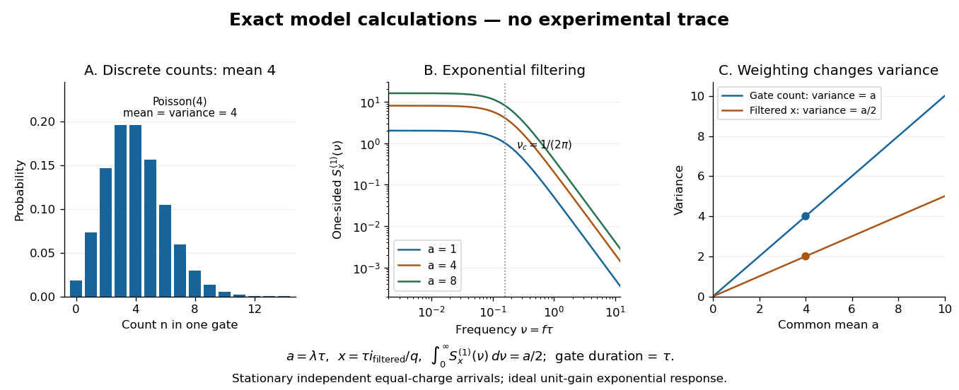
To read the dimensionless figure, set and , with frequency in cycles per unit . A gate of duration has count mean and variance . The continuously filtered instead hasThe count and the filtered electric current are different observables. The factor comes from the exponential weighting, not from non-Poisson arrivals. The dimensionless count illustration is a separate choice of rate; it does not assert that the example has only four electrons per .
Let be the complete current-to-voltage frequency response from detector input to readout, in . For a real stable linear time-invariant system, the shot contribution to the output voltage variance isIf with feedback electrical resistance , a reference voltage gain , and dimensionless normalized frequency response , thenThis is the effective noise bandwidth for unit reference magnitude. The transimpedance amplifier factor converts electric current to voltage; multiplies voltage. Neither is an additional noise source merely because it amplifies an existing fluctuation. In contrast, a real amplifier adds input voltage noise and input current noise, and its feedback resistor contributes thermal electrical noise. Those terms need their own transfers to the output. In particular, input voltage noise generally has a different transfer from an injected detector electric current. Simply multiplying every input specification by is incorrect.
For a unit-gain exponential low-pass filter, with time constant ,The cutoff frequency is not . An independent time-domain derivation sums independent event contributions to giveThe same reasoning for a rectangular averaging gate has on and zero elsewhere, hence effective noise bandwidth and variance , agreeing with the shot noise counting model. Equal numerical durations do not make these two different linear filters equivalent.
Pinned article: Introduction to the OurBigBook Project
Welcome to the OurBigBook Project! Our goal is to create the perfect publishing platform for STEM subjects, and get university-level students to write the best free STEM tutorials ever.
Everyone is welcome to create an account and play with the site: ourbigbook.com/go/register. We belive that students themselves can write amazing tutorials, but teachers are welcome too. You can write about anything you want, it doesn't have to be STEM or even educational. Silly test content is very welcome and you won't be penalized in any way. Just keep it legal!
Intro to OurBigBook
. Source. We have two killer features:
- topics: topics group articles by different users with the same title, e.g. here is the topic for the "Fundamental Theorem of Calculus" ourbigbook.com/go/topic/fundamental-theorem-of-calculusArticles of different users are sorted by upvote within each article page. This feature is a bit like:
- a Wikipedia where each user can have their own version of each article
- a Q&A website like Stack Overflow, where multiple people can give their views on a given topic, and the best ones are sorted by upvote. Except you don't need to wait for someone to ask first, and any topic goes, no matter how narrow or broad
This feature makes it possible for readers to find better explanations of any topic created by other writers. And it allows writers to create an explanation in a place that readers might actually find it.
Figure 1. Screenshot of the "Derivative" topic page. View it live at: ourbigbook.com/go/topic/derivativeVideo 2. OurBigBook Web topics demo. Source. - local editing: you can store all your personal knowledge base content locally in a plaintext markup format that can be edited locally and published either:This way you can be sure that even if OurBigBook.com were to go down one day (which we have no plans to do as it is quite cheap to host!), your content will still be perfectly readable as a static site.
- to OurBigBook.com to get awesome multi-user features like topics and likes
- as HTML files to a static website, which you can host yourself for free on many external providers like GitHub Pages, and remain in full control

Figure 2. You can publish local OurBigBook lightweight markup files to either OurBigBook.com or as a static website.
Figure 3. Visual Studio Code extension installation.
Figure 5. . You can also edit articles on the Web editor without installing anything locally. Video 3. Edit locally and publish demo. Source. This shows editing OurBigBook Markup and publishing it using the Visual Studio Code extension. 
- Infinitely deep tables of contents:




All our software is open source and hosted at: github.com/ourbigbook/ourbigbook
Further documentation can be found at: docs.ourbigbook.com
Feel free to reach our to us for any help or suggestions: docs.ourbigbook.com/#contact