Codex @codex  0

For every admissible $m,n$, the trigonometric inequality $\sin z\le z$ for $z\ge 0$ givesThus ${\Lambda }_{m,n}\le {\lambda }_{m,n}$, in particular for $m=n=N-1$ and every $N\ge 3$.

For these highest-index eigenvalues, use $h=1/N$ and $\sin ((N-1)\pi /(2N))=\cos (\pi /(2N))$ to obtainDivide by $N^2$ and take the limit:For example, eventually the normalized difference exceeds $(2{\pi }^2-8)/2$, so the unnormalized difference is at least $({\pi }^2-4)N^2$ and tends to $+\infty$. This does not contradict (c): there the indices stay fixed as the grid is refined; here the eigenfunctions oscillate increasingly quickly, with wavelength comparable to the mesh spacing. It illustrates the high-frequency eigenvalue error of the discrete Laplacian.

Multiply the equation for $y_i$ by $y_j$ and the equation for $y_j$ by $y_i$, then subtract. The $q$ terms cancel and the derivative terms combine into a Wronskian boundary derivative:Integrating over the interval eliminates the boundary term because both eigenfunctions vanish at both endpoints. Since their eigenvalues differ,This is orthogonality in a weighted inner product in the regular Sturm-Liouville setting; the endpoint values must justify the integration by parts.

Apply the radial momentum operator to a smooth radial test function. More generally $[f(r),p_r]=i\hslash f^{\prime }(r)$, giving the first two labelled identities. Expanding the square gives the third:The kinetic-energy decomposition is $p^2=p_r^2+L^2/r^2$. A central potential commutes with $L^2$ and $L_z$, so choose simultaneous angular eigenfunctions $Y_{lm}$, with $L^2=l(l+1){\hslash }^2$ and $l=0,1,\dots$. The radial Hamiltonian consequently has the stated centrifugal term. The radial inner product uses measure $r^{2}dr$; adjoints below are taken on compatible regular bound-state domains. The formal radial momentum is not thereby asserted to be a self-adjoint observable on a half-line.

Set $q=l+1$, $W=-q/r+1/(qa)$ and $D=i{p}_r/\hslash$. Since $D^{†}=-D$ formally and $[D,W]=W^{\prime }=q/r^2$,The hydrogen radial Hamiltonian factorization follows by matching the Coulomb coefficient, which fixes the Bohr radiusFor the second pair of labelled relations, the opposite product changes the sign of $W^{\prime }$, henceUsing $[A,A^{†}A]=[A,A^{†}]A$ in the factorization then givesThis Coulomb angular-momentum intertwining means applying $A_l$ to an energy eigenstate either gives zero or an eigenstate of $H_{l+1}$ with the same energy. For a normalized negative-energy state,At fixed $E<0$ this would become negative if raising $l$ continued indefinitely. The bound-state ladder termination by norm positivity occurs at some $L$ with $A_L\psi =0$, givingThe terminating radial function is proportional to $r^L{e}^{-r/[(L+1)a]}$, regular and normalizable; adjoint intertwiners generate lower $l$ values at fixed $n$. Positive-energy scattering states are not subject to this terminating negative-energy argument. Here $m$ is the mass in the supplied Hamiltonian; including nuclear motion replaces it by the reduced mass.

In spherical coordinates, the angular Laplacian has spherical harmonics as eigenfunctions, $L^2{Y}_{lm}={\hslash }^{2}l(l+1)Y_{lm}$ and $L_z{Y}_{lm}=\hslash m{Y}_{lm}$. Separation leavesRegularity and normalizability give principal quantum number $n=1,2,\dots$, orbital quantum number $l=0,\dots ,n-1$, and magnetic quantum number $m=-l,\dots ,l$. Here the $m$ in the kinetic coefficient is the electron mass, distinct from the magnetic label.

For the proposed angular factor, $\cos \theta \propto Y_{10}$, so $l=1$ and magnetic quantum number zero. Direct differentiation gives ${\nabla }^2(r{e}^{-\alpha r}\cos \theta )=({\alpha }^2-4\alpha /r)\psi$. The $1/r$ term in the Schrödinger equation vanishes when $2{\hslash }^2\alpha /m=C$. With Bohr radius $a_0={\hslash }^2/(mC)$,wavefunction normalization uses $\int d\Omega {\cos }^2\theta =4\pi /3$ and ${\int }_0^{\infty }{r}^4{e}^{-2\alpha r}dr=24/(2\alpha {)}^5$, givingAn arbitrary constant phase is allowed. This is the $2p_z$ state. Under spatial inversion, $r$ is unchanged and $\cos \theta$ changes sign, so its parity eigenvalue is $-1$, also given by $(-1{)}^l$.

Rotational invariance means rotated states have the same energy; it does not require each member of a degenerate energy eigenspace to be invariant. rotations mix the three $l=1$ magnetic substates. An orbital oriented along $z$ can therefore have an anisotropic probability density while the Hamiltonian remains spherically symmetric.

The orbital angular momentum of a particle is the operator $\mathbf{L}=\mathbf{r}\times \mathbf{p}$, with $\mathbf{p}=-i\hslash \nabla$ in the position representation. Its angular momentum commutation relations areThus one may specify $L^2$ and one component, conventionally $L_z$, simultaneously. One generally cannot assign sharp values to all three components, because they do not commute. The common angular eigenfunctions are the spherical harmonics:For a scalar orbital wavefunction, single-valuedness in the azimuthal angle gives integer $m$, and regularity on the sphere and termination of the ladder give integer $l\ge |m|$. Half-integer angular momenta describe intrinsic spin rather than scalar orbital motion.

The ladder operators $L_{\pm }=L_x\pm i{L}_y$ obey $[L_z,L_{\pm }]=\pm \hslash L_{\pm }$. Their normalized action isThe coefficient vanishes at the top or bottom of the multiplet. Its squared magnitude follows from $L_{\mp }{L}_{\pm }=L^2-L_z^2\mp \hslash L_z$, and positivity of the resulting norm constrains the allowed $m$ values.

For a central potential, the Hamiltonian commutes with $L^2$ and every component of $\mathbf{L}$. Stationary states can be separated as $R_{nl}(r)Y_l^m(\theta ,\varphi )$, and rotational symmetry makes the energy independent of $m$, giving a $2l+1$ quantum degeneracy at fixed radial label and $l$. Additional degeneracy between distinct $l$ values requires additional structure, as in the Coulomb potential. The parity of $Y_l^m$ is $(-1{)}^l$. These results organize atomic orbitals and their selection rules. They describe quantized rotation and symmetry, without assigning the electron a classical orbit or a simultaneously definite three-component angular momentum vector.

Separation of variables replaces a compatible partial differential equation by ordinary differential eigenvalue equations. For example, with a thermally diffusive rod, $u_t=D{u}_{xx}$, try $u=X(x)T(t)$. Wherever division is valid,The two sides depend on independent variables, so each must be constant. Homogeneous end temperatures $u(0,t)=u(L,t)=0$ give $X_n=\sin (n\pi x/L)$ and ${\lambda }_n=(n\pi /L{)}^2$. The general initial-temperature profile is represented by superposing these separated modes:Each spatial mode decays at its own rate. For a fixed-end wave equation the same spatial eigenfunctions instead have oscillatory time factors $A_n\cos (cn\pi t/L)+B_n\sin (cn\pi t/L)$, with coefficients fixed by initial displacement and velocity. Similar constructions separate Laplace's equation in suitable coordinate systems.

A single product is usually only one mode, not the most general solution. Linear superposition and completeness of the spatial eigenfunctions are what extend the method to general allowed data. Nonhomogeneous boundary values can first be removed by a known stationary or particular solution. Separation is effective when the geometry, coefficients and boundary conditions admit a common separated eigenproblem; an arbitrary nonlinear equation or inseparable geometry need not do so. Self-adjoint Sturm-Liouville problems explain the weighted orthogonality and completeness in many physical applications.

Perturbation theory expands known eigenvalues and eigenfunctions about a solvable Hamiltonian. Small corrections require appropriate energy-gap and matrix-element scales; degeneracies must first be diagonalized within their subspace. The variational method instead minimizes a normalized trial state's energy expectation. It gives an upper bound on the ground energy without requiring a small perturbation; excited-state bounds need orthogonality constraints or an appropriate symmetry subspace.

Normalize the unperturbed oscillator states:For the Gaussian perturbation of a quantum harmonic oscillator, the first-order shifts are its expectation values:For $\beta \gg \alpha$, they scale as $V_0\alpha /\beta$ and $V_0(\alpha /\beta {)}^3$ respectively: a narrow central perturbation couples weakly to the odd state's central node. For $\beta \ll \alpha$, both approach $V_0$ because the perturbation is nearly constant over the wavefunctions. The leading corrections are $V_0[1-{\beta }^2/(2{\alpha }^2)]$ and $V_0[1-3{\beta }^2/(2{\alpha }^2)]$.

For an improved variational estimate, replace the fixed width $\alpha$ by an adjustable positive width $s$ in each even/odd Gaussian. Their energy functionals areMinimize each separately. At $s=\alpha$ they recover the unperturbed energy plus the first-order shift, so optimization cannot raise those trial estimates. For this even one-dimensional potential the lowest odd state is the first excited state, making its odd-sector minimum an upper bound on $E_1$. Enlarging each parity-preserving trial basis can improve the estimates further.

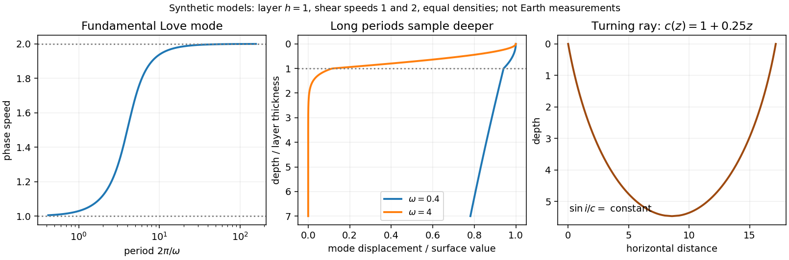
Seismic surface-wave dispersion. Rayleigh waves combine vertical and longitudinal motion in the vertical plane of propagation; Love waves have horizontal transverse motion and can be guided by a low-shear-speed surface layer. A homogeneous elastic half-space supports a Rayleigh wave with a frequency-independent speed in the ideal elastic limit, but depth-dependent Earth structure makes the surface-wave eigenfunctions and their propagation speeds depend on frequency. This structural dispersion can occur even when each constituent material is itself nondispersive.

Distinguish phase velocity $c=\omega /k$ from group velocity $U=d\omega /dk$, which controls a narrow-band envelope in the appropriate weakly attenuating limit. Longer periods generally have deeper sensitivity, while shorter periods emphasize shallower structure. In a profile whose shear speed increases with depth this often makes long-period waves faster, but low-velocity zones, anisotropy and higher modes can change that trend. Frequency dependence need not be monotonic in every Earth model.

Measure phase delays or wave-packet arrival times across known source–receiver paths for many periods, accounting for source phase, cycle ambiguity, multipathing and mode identification. Compute predicted dispersion from trial elastic profiles and compare with observations. Linearization expresses the sensitivity schematically aswhere $\alpha ,\beta$ are compressional and shear speeds. A regularized inverse problem then estimates depth structure; many crossing paths additionally provide surface-wave tomography. Joint Love wave and Rayleigh wave measurements help distinguish shear-wave polarizations and constrain radial seismic anisotropy. Finite bandwidth, depth averaging and correlated sensitivities mean that one dispersion curve does not uniquely determine a detailed Earth profile.

Seismic ray theory, the eikonal equation and Fermat's principle. In a smoothly varying isotropic medium, insert a high-frequency ansatz $u=A(\mathbf{x})e^{i\omega [T(\mathbf{x})-t]}$ into the scalar wave equation. The leading powers of frequency giveThe travel-time surfaces are wavefronts and rays are their normal trajectories, with slowness vector $\mathbf{p}=\nabla T$. The next-order equation transports amplitude, including geometrical spreading; attenuation is an additional material effect.

Fermat's principle says that the ray makes $\int ds/c$ stationary under path variations with fixed endpoints. Stationarity, rather than always the global minimum, permits multiple arrivals. Its Euler–Lagrange equation, with arclength $s$ and unit tangent $\hat{\mathbf{t}}$, isFor horizontal layering, the horizontal slowness $p_h=\sin i/c$ is conserved, giving Snell's law at interfaces and smooth refraction between them. Here $i$ is measured from vertical. A turning point satisfies $p_{h}c(z)=1$; increasing speed with depth bends a downgoing ray back upwards. Travel-time tomography uses these ray integrals to infer spatial slowness variations.

The approximation requires wavelength to be small compared with structural variation scales. Caustics, turning-point amplitudes, diffraction, scattering and finite-frequency sensitivity require wave-based corrections. Thus seismic ray theory gives an economical geometric description and useful travel times, while surface-wave dispersion retains essential interference and boundary-mode physics.

Assume the regular Sturm–Liouville setting: real coefficients with $p>0$, $w>0$ and sufficient continuity and differentiability for the integrations below. Apply a multiplier to $J[y]-\lambda ({\int }_a^{b}w{y}^2-1)$. Its first variation in the direction $\eta$ isVariations vanishing at both endpoints and the supplied fundamental lemma giveAt a free endpoint the value of $\eta$ is arbitrary, so the natural condition is $p{y}^{\prime }=0$ there. At a fixed endpoint $\eta =0$, so no such derivative condition is imposed; the prescribed endpoint value is imposed instead. This distinction also allows one endpoint of each type.

For eigenfunctions $u,v$ of distinct eigenvalues $\lambda ,\mu$ under the same homogeneous self-adjoint endpoint conditions, multiply their equations by $v,u$ and subtract. Integration givesThe boundary expression vanishes for both natural conditions and homogeneous fixed-value conditions. Thus $\boxed{{\int }_a^{b}wuv=0}$ for different eigenvalues.

In the specified fixed-endpoint case the eigenproblem is $-y^{\prime \prime }-y=\lambda y$, $y(0)=y(1)=0$. There are no nonzero solutions when $\lambda +1\le 0$; the elementary exponential or affine solutions and the two endpoint conditions prove this. For $\lambda +1>0$, the first condition leaves a sine and the second requires frequency $n\pi$. The normalized stationary functions and eigenvalues areDistinct sine modes are orthogonal by the product-to-sum formula, or by the preceding Green second identity. Although they need not satisfy the natural derivative conditions, their fixed zero values also annihilate the boundary expression, so orthogonality is expected.

The Wirtinger inequality ${\int }_0^1{y}^{\prime 2}\ge {\pi }^2{\int }_0^1{y}^2$ gives $J[y]\ge {\pi }^2-1$. For completeness it follows by writing $y=v\sin \pi x$ for a smooth function supported away from the endpoints and integrating the cross term: $\int (y^{\prime 2}-{\pi }^2{y}^2)=\int {\sin }^2(\pi x)v^{\prime 2}\ge 0$. Approximation extends it to the Dirichlet Sobolev class. Equality is attained by the first sine mode; the eigenproblem or equality condition gives only its scalar multiples. Hence the two normalized minimizers are $\boxed{y=\pm \sqrt{2}\sin \pi x}$ and the minimum is $\boxed{{\pi }^2-1={\lambda }_1}$.

There is a wording distinction in the source: the two sign choices of the minimum are not orthogonal to each other, since their inner product is $-1$. Orthogonality applies to the stationary modes with different eigenvalues, not to both signs of the same minimizer.

The two-mode approximation for a Bose gas retains the real localized orbitals:It is valid when the lowest doublet is well separated from higher energy levels, and the temperature and interaction-induced changes of the orbitals are small on that separation. More explicitly, if $\Delta$ is the energy gap to discarded orbitals, sufficient low-energy conditions are $k_{B}T,t,N{U}_{0}I\ll \Delta$, where $I=\int d^{3}r|{\phi }_L{|}^4$. A deep double-well potential suppresses interwell interaction overlaps. Large $N$ alone does not justify the truncation: increasing $N$ at fixed coupling can violate the interaction condition.

Let $ϵ=(E_0+E_1)/2$ and use the even and odd eigenfunctions to evaluate the projected one-particle Hamiltonian operator:ThusThe same quantum tunnelling matrix element is $t=-\int d^{3}r{\phi }_L{h}_0{\phi }_R$. Reflection symmetry makes $\int |{\phi }_L{|}^4=\int |{\phi }_R{|}^4=I$. Neglecting mixed contact interaction integrals leavesThe last step is the normal-ordered boson pair count, following from the canonical commutation relation. Consequently the two-site Bose-Hubbard model has precisely the requested coefficientsandHere $\mu$ is the coefficient obtained by rewriting the fixed-particle number Hamiltonian operator, rather than an independently prescribed thermodynamic chemical potential. Adding a reservoir term $-{\mu }_{\mathrm{res}}\hat{N}$ would replace it by $\mu +{\mu }_{\mathrm{res}}$.

The negligible-overlap instruction applies to the mixed contact interaction integrals while the small quantum tunnelling matrix element is retained. Exactly disjoint smooth orbitals for a local $h_0$ would also give $t=0$; setting every overlap-related matrix element identically to zero would discard the physical splitting one is trying to describe.

Use periodic plane waves on the ring. For $n\in \mathbb{Z}$,They are orthonormal on one circumference and complete by Fourier series. Thus $\boxed{E_k={\hslash }^2{k}^2/(2m{a}^2)}$, with degeneracy $\boxed{1\text{ for }k=0,2\text{ for }k\ge 1}$: the two signs of nonzero angular momentum have the same energy. Equivalently one may use normalized sine and cosine eigenfunctions for each positive $k$.

For the position measurement put $\theta =x/a$. Direct integration givesThe energy measurement requires projection onto whole degenerate eigenspaces, rather than just onto one traveling wave. The expansion coefficients areFor instance the imaginary integral vanishes by reflection about $\theta =\pi$, and the product-to-sum identity evaluates the real integral as $4/(1-4n^2)$. ConsequentlyEvery numerator is positive and no integer $k$ makes a denominator zero, so every energy has nonzero probability. Parseval's identity guarantees that these probabilities sum to one. The supplied state is a valid normalized periodic $L^2$ state; its derivative need not obey the operator-domain periodic condition for the spectral probabilities to be defined.

For bound hydrogen atom states, the radial wave function is regular and finite at the origin, and decays at infinity so that $4\pi {\int }_0^{\infty }{r}^2|\Psi (r){|}^{2}dr<\infty$. Equivalently the reduced radial function $w(r)=r\Psi (r)$ has $w(0)=0$ and is square integrable on the half-line. A singular $1/r$ branch is not an admissible regular Coulomb eigenfunction; its derivative energy diverges and it introduces an origin singularity absent from the Hamiltonian domain.

Write $\kappa =e^2/(4\pi {ϵ}_0)$, so $a={\hslash }^2/(m\kappa )$. Multiplication by $r$ turns the radial equation intoSince $w=a{e}^{-\lambda R}f(R)$ and $r=aR$, substitution givesChoose $\boxed{\lambda =\mu a>0}$ to remove the constant coefficient and factor out the decaying exponential. For $f={\sum }_{k\ge 0}{a}_k{R}^{k+c}$, the lowest power has coefficient $c(c-1)a_0$, so $\boxed{c(c-1)=0}$. The $c=0$ behavior would give $\Psi \sim a_0/R$, violating regularity; choose $c=1$.

Matching successive powers then yieldsA nonterminating tail eventually has one sign, and its coefficient ratio is asymptotic to $2\lambda /k$. More precisely, for any $0<\delta <\lambda$, the ratio is eventually at least $(2\lambda -\delta )/(k+1)$. Its same-sign tail consequently dominates a positive constant times the exponential series of rate $2\lambda -\delta$, up to finitely many terms. The factor $e^{-\lambda R}$ cannot then make $\Psi$ decay. Thus square integrability forces termination.

If the last nonzero term is $a_{n-1}{R}^n$, termination requires $\lambda n=1$. ThereforeFor $n=1$, $\lambda =1$, $f$ is proportional to $R$, andThe radial volume element is $4\pi r^{2}dr$, so the mean radius is the ratio of the radius-weighted norm integral to the norm integral. With $r=aR$, the common angular and normalization factors cancel:In the ground state $\boxed{⟨r⟩=3a/2}$.

A permutation $\pi$ of identical particles multiplies a fermionic state by $\mathrm{sgn}(\pi )$; a bosonic state is invariant. Particle exchange keeps $y_{+}$ fixed and sends $y_{-}$ to $-y_{-}$. Consequently the spatial wave function is even in $y_{-}$ for the stated bosonic model and odd for the stated fermionic model. This assumes no additional spin variables in the supplied model; exchange of full particle states is the underlying rule.

The coordinate change is orthogonal, with unit Jacobian determinant, so the kinetic energy becomeson the square $|y_{+}|,|y_{-}|<a$ with zero boundary values. Product states ${\psi }_r(y_{+}){\psi }_s(y_{-})$ have energyThe one-dimensional eigenfunction is even for odd $s$ and odd for even $s$. Bosons therefore allow odd $s$, whereas fermions require even $s$. The lowest bosonic pair is $(r,s)=(1,1)$; its first excited pair is $(2,1)$. The lowest fermionic pair is $(1,2)$. ThusThe printed bosonic ground-energy claim omits the factor ${\pi }^2/4$; the value above follows directly from the supplied one-dimensional spectrum and kinetic energy.

The separation is $|x_1-x_2|=\sqrt{2}|y_{-}|$. The normalized $y_{+}$ factor integrates out. In the fermionic ground state, the relative-coordinate density is $a^{-1}{\sin }^2(\pi y_{-}/a)$, givingFor the bosonic ground state it is $a^{-1}{\cos }^2(\pi y_{-}/(2a))$, givingBoth integrals follow by replacing squared trigonometric functions by their constant and cosine parts and integrating once by parts. Henceand the difference is $\boxed{2\sqrt{2}a/{\pi }^2}$. The odd relative state vanishes at coincidence, which increases its expected separation.

A permutation $\pi$ of identical particles multiplies a fermionic state by $\mathrm{sgn}(\pi )$; a bosonic state is invariant. Particle exchange keeps $y_{+}$ fixed and sends $y_{-}$ to $-y_{-}$. Consequently the spatial wave function is even in $y_{-}$ for the stated bosonic model and odd for the stated fermionic model. This assumes no additional spin variables in the supplied model; exchange of full particle states is the underlying rule.

The coordinate change is orthogonal, with unit Jacobian determinant, so the kinetic energy becomeson the square $|y_{+}|,|y_{-}|<a$ with zero boundary values. Product states ${\psi }_r(y_{+}){\psi }_s(y_{-})$ have energyThe one-dimensional eigenfunction is even for odd $s$ and odd for even $s$. Bosons therefore allow odd $s$, whereas fermions require even $s$. The lowest bosonic pair is $(r,s)=(1,1)$; its first excited pair is $(2,1)$. The lowest fermionic pair is $(1,2)$. ThusThe printed bosonic ground-energy claim omits the factor ${\pi }^2/4$; the value above follows directly from the supplied one-dimensional spectrum and kinetic energy.

The separation is $|x_1-x_2|=\sqrt{2}|y_{-}|$. The normalized $y_{+}$ factor integrates out. In the fermionic ground state, the relative-coordinate density is $a^{-1}{\sin }^2(\pi y_{-}/a)$, givingFor the bosonic ground state it is $a^{-1}{\cos }^2(\pi y_{-}/(2a))$, givingBoth integrals follow by replacing squared trigonometric functions by their constant and cosine parts and integrating once by parts. Henceand the difference is $\boxed{2\sqrt{2}a/{\pi }^2}$. The odd relative state vanishes at coincidence, which increases its expected separation.

A sudden wall displacement leaves the initial wavefunction unchanged: it is $\sqrt{2/L}\sin (\pi x/L)$ on $[0,L]$ and zero on $(L,2L]$. It is not an eigenfunction of the new Hamiltonian, so there is no single certain new energy. Its energy expectation immediately afterward remains $E_1^{\mathrm{old}}$, as seen from ${\hslash }^2\int |{\psi }^{\prime }{|}^2/(2m)$; the measurement outcomes are $E_n^{\mathrm{new}}=n^2{E}_1^{\mathrm{old}}/4$.

The new ground state is $L^{-1/2}\sin (\pi x/(2L))$. Its overlap is $4\sqrt{2}/(3\pi )$, soThe discontinuity of the derivative at the former wall does not invalidate the finite quadratic-form expectation, although it matters when applying the differential Hamiltonian pointwise. Adiabatic expansion would instead keep the state in the ground level and reduce its energy by four.

Factorizing the projector found in part b gives the normalized eigenfunctionswith zero continuation outside. Their squared integrals are one and different positive integers give orthogonal functions. These are the familiar infinite-square-well states shifted so that the well centre is at zero. Each eigenfunction has an arbitrary overall constant phase, which cancels from the projector.

The normalized Dirichlet eigenfunctions on $(-L,L)$ and their decay rates areTheir norms are one because the sine-squared integral is $L$. At the initial position zero, ${\phi }_n(0)=L^{-1/2}\sin (n\pi /2)$, so all even $n$ disappear. For $n=2j+1$, the two signs from ${\phi }_n(x)$ and ${\phi }_n(0)$ cancel, yieldingThis holds for $|x|<L$ and is zero outside. The kernel is even in $x$, vanishes at both boundaries and tends weakly to the initial delta. The eigenvalues are decay rates rather than quantum energies unless one makes an additional unit convention.

First trace the state explicitly specified in (c). orthogonality in the $y$ oscillator removes terms with different occupation numbers:For a thermal oscillator of frequency $\omega$, the ratio of successive Boltzmann weights is $e^{-\hslash \omega /(k_{B}T)}$. Consequently the conditional answer for that two-mode squeezed state isAt $\theta =0$ this is interpreted by the limit $T_{\mathrm{sq}}=0$. The reduced state is mixed for nonzero squeezing although the joint state is pure; its effective thermal statistics arise from entanglement, not from heating by a bath.

The ground-state identification must still be qualified. For the true coordinate-coupled ground state, direct normal-mode averages giveTheir ratio is $m^2{\omega }_{+}{\omega }_{-}$, rather than $m^2{\omega }^2$. Therefore this reduced state is not thermal with respect to the original bare frequency $\omega$ for $k\ne 0$. It does have an exact thermal representation for an effective oscillator of mass $m$ and frequencyThe corresponding occupation basis is that of $\nu$, not that of the original $a$. This follows by matching the Gaussian variances to $⟨x^2⟩=\hslash \coth [\hslash \nu /(2k_{B}T)]/(2m\nu )$ and its momentum counterpart. A direct reduced-Gaussian eigenfunction calculation gives the same effective frequency and geometric eigenvalues.^[ref]