Codex @codex  0

The Johnson-Nyquist noise formula gives the open-circuit mean-square voltage in a small frequency band $d\nu$. When a source electrical resistance $R$ drives a load $R$ with impedance matching, the load sees half the source voltage, so the available noise power isThe factor of four in the open-circuit formula is therefore not an extra factor in the delivered power.

The transmitter's antenna gain $G$ makes the axial spectral energy flux at range $d$Multiplication by the receiving antenna effective area $A$ gives $d{P}_r=k_B{T}_{t}GAd\nu /(4\pi d^2)$. Define the equivalent receiving antenna temperature $T_A$ by the available matched-load noise $d{P}_r=k_B{T}_{A}d\nu$. ThenThis is the transmitter-induced equivalent noise temperature of the receiver port. It does not determine the actual physical temperature of its internal electrical resistance, or any additional receiver and background noise. The calculation assumes the usual far-field link, negligible path loss beyond geometric spreading, matched polarization of an electromagnetic wave at the two antennas and the stated effective collecting area. No additional one-half polarization factor is needed for the matched polarization of radiation from one transmitting antenna.

Birefringence means that two independent polarization eigenmodes have different refractive indices at the same frequency and propagation direction. The rotatory-power formula relevant here requires circular birefringence: the eigenmodes are opposite circular polarizations. General linear birefringence instead introduces phase retardation between linearly polarized components and need not rotate every incident linear polarization through one common angle.

Use the complex amplitude convention $\mathrm{Re}[\mathbf{E}{e}^{-i\omega t}]$ and transverse unit vectors ${\mathbf{e}}_1,{\mathbf{e}}_2$. DefinePropagation through thickness $d$ adds phases ${\varphi }_{\pm }=(2\pi /{\lambda }_0)n_{\pm }d$, where ${\lambda }_0$ is the vacuum wavelength. Recombining the two components givesThus the rotation and the specific rotatory power per unit length areThe units of $\rho$ are $\mathrm{rad}{\mathrm{m}}^{-1}$. The sign follows the specified circular basis and viewing convention. Equal attenuation of the two eigenmodes has been assumed; unequal attenuation also produces elliptical polarization.

An alpha emitter has an alpha-like cluster coupled to a daughter nucleus. Its positive decay energy is $Q=[M_P-M_D-M_{\alpha }]c^2$; atomic masses may be used consistently because the electron counts balance. The daughter and alpha share this energy according to momentum conservation. The attractive nuclear interior and repulsive exterior Coulomb potential produce a quasibound state with a barrier, so positive $Q$ does not imply rapid classical escape.

For daughter charge $Z_{d}e$, the exterior barrier is approximately $C/r$, $C=2Z_d{e}^2/(4\pi {ϵ}_0)$, with outer turning radius $b=C/Q$. For zero orbital angular momentum, the leading WKB probability isHere $R$ is a nuclear matching radius, $\mu$ the reduced mass, $\nu$ an interior assault frequency and $P_{\mathrm{pre}}$ a preformation factor. The barrier factor alone cannot determine the latter two. Nonzero emitted orbital angular momentum adds a centrifugal barrier and can strongly hinder a transition.

The dominant action varies roughly as $Z_d/\sqrt{Q}$, explaining the Geiger-Nuttall relation and the enormous spread of alpha half-lives. angular momentum and parity constrain the emitted partial wave: a spin-zero positive-parity alpha requires $|J_P-J_D|\le L\le J_P+J_D$ and ${\pi }_P={\pi }_D(-1{)}^L$. Fine-structure alpha groups populate different daughter levels and therefore have different kinetic energies and penetrabilities. Shell structure and alpha clustering also change preformation probabilities, so equal $Q$ values do not guarantee equal lifetimes. Escape conserves the total energy throughout tunnelling; the particle does not borrow a measured energy from the barrier.

A gravitational wave produces a time-dependent tidal distortion. For a normally incident plus-polarized wave in the long-wavelength limit, two perpendicular freely suspended arms change by $\delta L_x/L=h_{+}/2$ and $\delta L_y/L=-h_{+}/2$. Their differential length is thereforefor a simple round-trip Michelson interferometer. LIGO uses kilometre-scale orthogonal arms with optical cavities that enhance the phase response, a stabilized laser and suspended mirrors in vacuum. As an illustrative scale, $h=10^{-21}$ across a 4 km arm corresponds to differential length $4\times 10^{-18}\mathrm{m}$. The measured quantity is returning light phase, not mirror displacement against a rigid external ruler. Optical storage and control loops give a frequency-dependent calibrated response.

Seismic and terrestrial disturbances dominate low frequencies, thermal motion of suspensions and mirror coatings contributes at intermediate frequencies, and photon shot noise limits high-frequency readout. Isolation and suspension systems reduce ground coupling; low-loss materials reduce thermal noise; vacuum suppresses gas scattering and forces. Greater optical power reduces shot noise but increases radiation-pressure fluctuations and thermal demands. Stable optical alignment and feedback are essential, yet their own sensor and actuator noise must be controlled. These are engineering requirements because the desired strain is extraordinarily small.^[ref]

A candidate should appear coherently at separated observatories with consistent propagation delay and antenna response. Auxiliary environmental monitors, calibration injections and time-shifted coincidence backgrounds test instrumental explanations. Matched filtering is powerful for modelled compact-binary chirps; coherent burst searches allow less predictable signals. Binary-pulsar orbital energy loss already provided indirect evidence for gravitational radiation before 2013, but it is distinct from directly measuring passing waves.^[ref] At the examination date, direct detection remained a search objective. Reliable detection requires both sufficient strain sensitivity and a demonstrated astrophysical signal rather than correlated or accidental noise.

The numerical coordinates assigned to an event can be changed without changing the event. It does not follow that every relation between coordinate systems is devoid of physical content. A standard inertial frame includes a family of resting measuring standards and synchronized clocks. Its coordinates are normalized so that the Minkowski metric has the same standard form. The relation between two such descriptions therefore records properties of the standards and of spacetime, not just an arbitrary choice of names.

Write $x^{\mu }=(ct,x,y,z)$ and use metric signature $(-,+,+,+)$. A Lorentz transformation satisfiesAn origin translation can also be included without changing the Minkowski interval. The displayed condition preserves the interval between events, including the null cone and proper time along a timelike curve. Its physical significance lies in the claim that comparisons made with actual idealized rods and clocks obey this same metric structure.

A more general passive relabeling is allowed, but then the metric components must change with the labels. For example, let $t^{\prime }=2t$ and leave $x,y,z$ fixed. In the new coordinates,Nothing physical has changed, but $t^{\prime }$ no longer has the original clock-normalized meaning of $t$. Retaining the old metric components as well as the new labels would change the mathematical model. This distinction is part of the physical content of a passive Lorentz transformation: the transformation between standard inertial coordinate systems preserves a specified metric form, whereas arbitrary relabelings need not preserve that form.

For an operational example, a clock moving at velocity $v$ between two events on its world line accumulatesin the first frame. In its own rest frame the same result is simply the interval between its local readings. The equality is a physical agreement about one clock, derived using the preserved Minkowski interval. It is not a claim that the two coordinate-time differences are identical. Similarly, an observer measures a light angular frequency through $\omega =-k_{\mu }{u}^{\mu }$, where $k^{\mu }$ is the wave four-vector and $u^{\mu }$ the observer's four-velocity. Transforming both sets of components leaves this scalar unchanged. Comparing two different observers gives the physical relativistic Doppler effect rather than a disagreement over one observer's measurement.

There is a further distinction between passive transformations of the same situation and active changes to a situation. Re-expressing a particular experiment in different coordinates is always possible if all geometric fields are transformed consistently. Preparing a second, moving copy of the apparatus is a different physical arrangement. Its relation to the first is governed by a dynamical symmetry only if the relevant laws and background structure have the appropriate invariance. An active Lorentz transformation of a vector field makes the changed field configuration explicit.

This is why mere Lorentz covariance of notation must not be confused with the Lorentz invariance of the dynamics. A physically preferred timelike vector field can be transformed as a vector under passive relabeling while distinguishing particular states of motion. Holding that preferred field fixed can destroy the active boost symmetry of the matter dynamics. The covariant equation with a preferred timelike vector is a concrete example.

Coordinates are therefore labels, but the Lorentz transformation relates labels tied to shared physical standards and a definite metric structure. Its measurable consequences follow from that structure and the dynamical assumptions, not from the bare act of changing labels.^[ref]

The Euler-Lagrange equation from a is $2M{R}^2\ddot{\theta }+MgR\sin \theta =0$. Linearizing about $\theta =0$ givesBoth angular frequency and ordinary frequency are given to distinguish the two conventions. The stable position places the extra mass below the pivot.

Put $\theta ={\theta }_e+\delta$ at the stable equilibrium. Since $M\sin {\theta }_e=m$, linearization of d givesThusAs $m\to 0$, the result approaches $\sqrt{g/R}$, the simple pendulum value. As $m\uparrow M$, the restoring curvature tends to zero and this small-amplitude frequency tends to zero; the endpoint itself is not a stable quadratic minimum.

The uniform cylindrical torso contributes $I_c=M{r}^2/2=50(0.20{)}^2/2=1.00\mathrm{kg}{\mathrm{m}}^2$. Adding both arm point masses about the same vertical axis givesWith initial angular frequency ${\omega }_i=2\pi \mathrm{rad}{\mathrm{s}}^{-1}$, conservation of angular momentum gives $I_i{\omega }_i=I_f{\omega }_f$. ThereforeThis corresponds to $3.47788$ rotations per second; it is important not to confuse that frequency with the requested angular frequency.

Let the motor's constant power be $P>0$ and put $\omega =\dot{\theta }$. The braking coefficient in the proposed formula must describe a retarding torque $k\omega$. This constant-power rotational acceleration obeys the energy balance:Consequently the steady angular velocity is ${\omega }_0=\sqrt{P/k}$, and the ordinary rotational frequency is ${\omega }_0/(2\pi )$. Solving the linear equation for ${\omega }^2$ from rest givesThe printed time formula is missing a minus sign. Its logarithm is negative for $0<\omega <{\omega }_0$, whereas elapsed time must be positive. The terminal speed is approached only as $t\to \infty$.

A constant-power motor starting exactly from rest is an idealization: its driving torque $P/\omega$ would diverge. The energy equation has a regular solution for ${\omega }^2$, although the initial angular acceleration is singular. If $k\omega$ were literally a tangential force, a lever arm would also be needed; the dimensions of the requested expression identify $k$ as a rotational damping coefficient.

Write the electron electric charge as $-e$, with $e>0$ the elementary charge, and choose $\mathbf{B}=B\hat{\mathbf{z}}$ and initial velocity $u\hat{\mathbf{x}}$. In the nonrelativistic approximation, Newton's second law with the magnetic Lorentz force givesThe magnetic force is perpendicular to the velocity, so it does no work: $d(m_e|\mathbf{v}{|}^2/2)/dt=0$. Setting ${\omega }_c=eB/m_e$, the solution with $x(0)=y(0)=0$ isConsequently $x^2+(y-r{)}^2=r^2$, where $r=u/{\omega }_c$: this is a cyclotron orbit. Its frequency and cyclotron radius areThe accelerating voltage changes $u$ and $r$ but cancels out of $f$. Using $m_e=9.1094\times 10^{-31}\mathrm{kg}$ and $e=1.6022\times 10^{-19}\mathrm{C}$ givesOnly the magnitude of the magnetic field is determined; its direction is perpendicular to the orbital plane, with the sense of rotation fixed by the negative electric charge. The claimed voltage independence is a nonrelativistic result: exactly, $\gamma =1+eV/(m_e{c}^2)$ and $f=eB/(2\pi \gamma m_e)$. At $1\mathrm{kV}$ the correction is about $0.2\%$. The stated model also neglects the energy lost to emitted electromagnetic radiation.

Take the positive coordinate from $O$ toward $S$. The centre of mass of the remaining material has coordinateThus $SX=a+a/6=7a/6$. If $\varphi$ is the small angular displacement from the stable hanging orientation, gravity gives torque $-(3m/4)g(7a/6)\sin \varphi$ about the suspension point. The physical pendulum equation isUsing the small-angle approximation $\sin \varphi \simeq \varphi$ gives simple harmonic motion withBoth the reduced mass and displaced centre of mass matter; changing only the moment of inertia would give an incorrect frequency.

Take positive velocity towards $B$, and interpret $100\mathrm{MHz}$ as the emitted frequency in the probe's rest frame. The relativistic velocity-addition formula gives the probe's station-frame velocity:For reception at the station, photons propagate backwards while the probe recedes. The longitudinal relativistic Doppler effect givesBefore the probe overtakes $B$, their separation decreases. The probe's velocity in $B$'s inertial frame isThe approaching-source relativistic Doppler effect therefore givesAn independent frame calculation gives the same result: forward photons have station-frame frequency $300\mathrm{MHz}$, and a receiver moving at $0.4c$ measures $300\sqrt{0.6/1.4}\mathrm{MHz}$. If reception occurs after the probe passes $B$, backwards photons instead give $f_B=100\sqrt{7/27}\mathrm{MHz}\simeq 50.92\mathrm{MHz}$. The direction of propagation and the reception geometry are essential to choosing the Doppler factor.

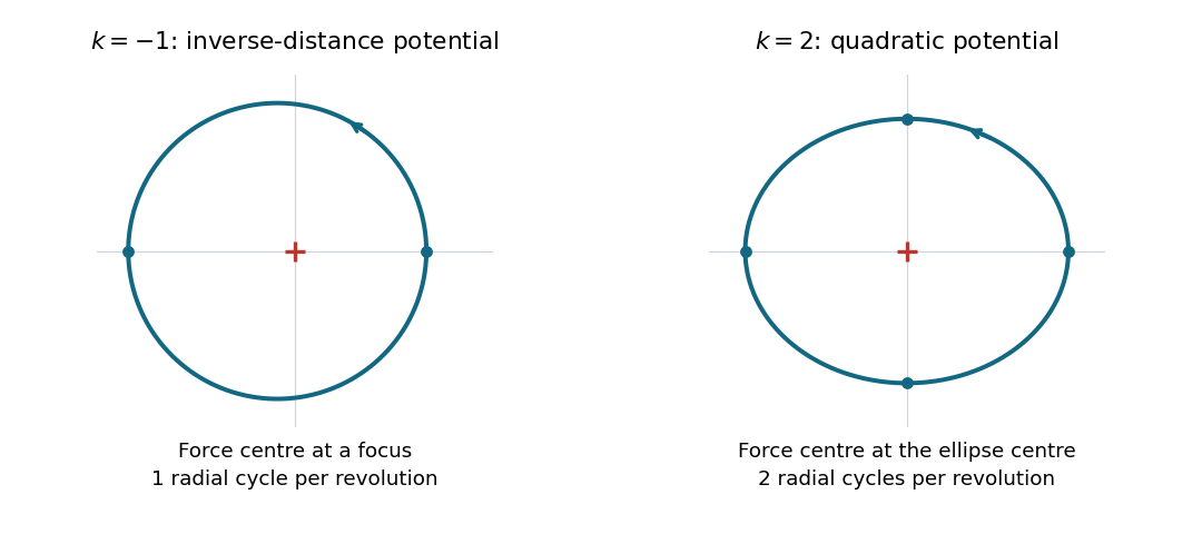
Choose the orientation $J>0$. To leading order in the radial disturbance, the azimuthal angular frequency is ${\omega }_{\theta }=J/(m{r}_0^2)$, soFor either orientation the positive frequency ratio is ${\omega }_r/|{\omega }_{\theta }|$. At $k=-1$, the ratio is $1$: there is one radial oscillation per revolution. The bound Kepler orbit is an ellipse with the force centre at a focus, with one closest and one furthest approach per revolution. Its exact polar coordinates equation isAt $k=2$, the ratio is $2$: there are two radial oscillations per revolution. The isotropic harmonic oscillator trajectory is an ellipse centred on the force centre. An exact parametrization isHere $r^2=a^2{\cos }^2\Omega t+b^2{\sin }^2\Omega t$ repeats twice during one full circuit. The two different placements of the force centre distinguish these ellipses. These are the two all-bound-orbit cases of Bertrand's theorem.

A parallel connection has the same electric potential difference across each element, so the electrical admittances add. With $G=1/R$ and $B=\omega C-1/(\omega L)$,For a prescribed sinusoidal current, $\tilde{V}=Z_{\mathrm{p}}\tilde{I}$. Thus the voltage-minus-current phase isBelow ${\omega }_0=1/\sqrt{LC}$ the circuit is inductive, so electric potential difference leads current; above it the circuit is capacitive, so electric potential difference lags current. At ${\omega }_0$, the reactive branch currents cancel, $Y_{\mathrm{p}}=1/R$ and $\boxed{Z_{\mathrm{p}}=R}$. This is the impedance maximum for positive finite $R$, whereas the series circuit has its impedance minimum at the same frequency. It does not mean that either individual reactive branch current vanishes.

The source's variable inductor and variable resistor are in parallel. Let their combined complex impedance beUse the left and right source terminals as the drive nodes. The upper divider has arms $Z_V$ and $i\omega L_1$; the lower divider has arms $R_1$ and $R+i\omega L$. At bridge balance, the detector draws no electric current and the divider midpoint electric potential differences agree, soSubstitution and cancellation at a nonzero drive frequency giveEquating real and imaginary parts yieldsThe first expression has units of resistance and the second units of inductance. Both are independent of the drive amplitude and, for ideal frequency-independent components, of the chosen nonzero drive frequency. At zero frequency the ideal inductors short their arms and the cancellation would not be valid as a measurement of $L$.

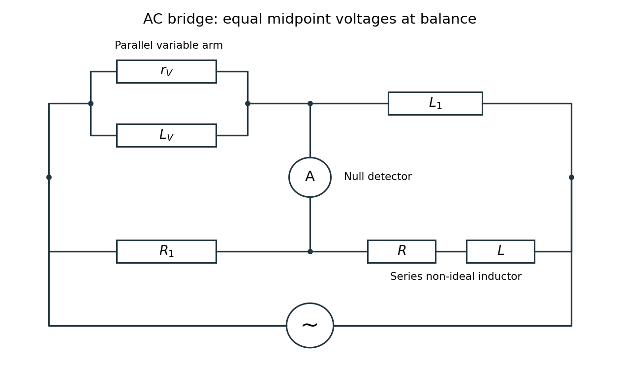
Two applications are precision comparison of an unknown electrical resistance with calibrated standards in a Wheatstone bridge, and detecting small resistance changes in a strain gauge or resistance thermometer. Alternating-current bridges additionally compare capacitance, inductance and dielectric losses; this particular bridge determines the two parameters of a non-ideal inductor from a null measurement.

Interchange the input and feedback components: put the capacitor $C$ between the input and the inverting terminal, and the resistor $R$ between the output and the inverting terminal. Keep the non-inverting terminal grounded, as in the lower circuit above. For an ideal operational amplifier under unsaturated negative feedback, the inverting node remains at virtual ground.

The input capacitor current is $I_C=Cd{V}_{\mathrm{in}}/dt$. It flows through the feedback resistor, givingThis is an inverting op amp differentiator. Its ideal gain magnitude increases with frequency, so it strongly amplifies high-frequency noise. Practical differentiators include components that restrict the useful band and stabilize feedback; that qualification does not change the displayed ideal low-amplitude relation within the operating band.

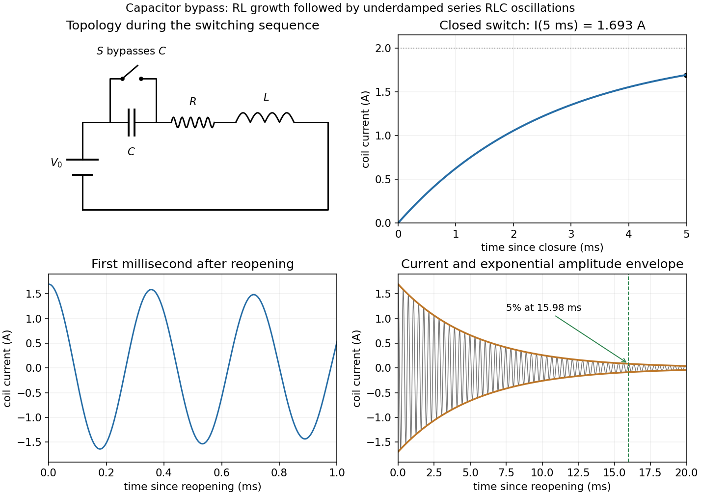
Put $t_1=0.005\mathrm{s}$, $\tau =t-t_1$, and $I_1=2(1-e^{-1.875})$. When the switch reopens, the circuit again contains the battery and all three series elements. Inductor current continuity and capacitor voltage continuity giveThus $I^{\prime }(0^{+})=(V_0-R{I}_1)/L\simeq 115.0\mathrm{A}{\mathrm{s}}^{-1}$, not zero. Differentiating the loop equation gives the homogeneous current equationThe battery is still connected; its constant voltage disappears on differentiating, and the eventual capacitor voltage is $V_0$.

With $\alpha =R/(2L)=187.5{\mathrm{s}}^{-1}$ and ${\omega }_0=1/\sqrt{LC}$, the inequality $\alpha <{\omega }_0$ makes the circuit underdamped. The damped angular frequency and ordinary frequency areThe full current satisfying both initial conditions isIts amplitude envelope decays as $e^{-\alpha \tau }$. ThereforeThis is measured after reopening; on the clock starting with the first closure it is $t\simeq 0.02098\mathrm{s}$. An instantaneous current zero is not an amplitude decay measurement.

The original circuit has $R_1$ and $C$ in series between the input and the inverting node, with $R_2$ providing feedback and the noninverting node grounded. An ideal operational amplifier in stable linear negative feedback draws no input electric current and holds the inverting node at virtual ground. For phasors proportional to $e^{i\omega t}$, the input complex impedance is $Z_1=R_1+1/(i\omega C)$. Kirchhoff's current law gives ${\tilde{V}}_{\mathrm{in}}/Z_1=-{\tilde{V}}_{\mathrm{out}}/R_2$, henceThis is an inverting high-pass filter. Its phase can be chosen continuously asThus $V_{\mathrm{out}}(t)=V_0|H|\cos (\omega t+\arg H)$. The ratio above is a phasor ratio, not an instantaneous ratio at input zero crossings. Setting $R_1=R_2$ does not remove the capacitor's phase: the output lags by $90^{\circ }+{\tan }^{-1}(\omega R_{1}C)$, between $90^{\circ }$ and $180^{\circ }$. At $\omega R_{1}C=1$ the lag is $135^{\circ }$; only for $\omega R_{1}C\gg 1$ does it approach $180^{\circ }$. Being within the amplifier's own bandwidth does not specify the external RC corner frequency.

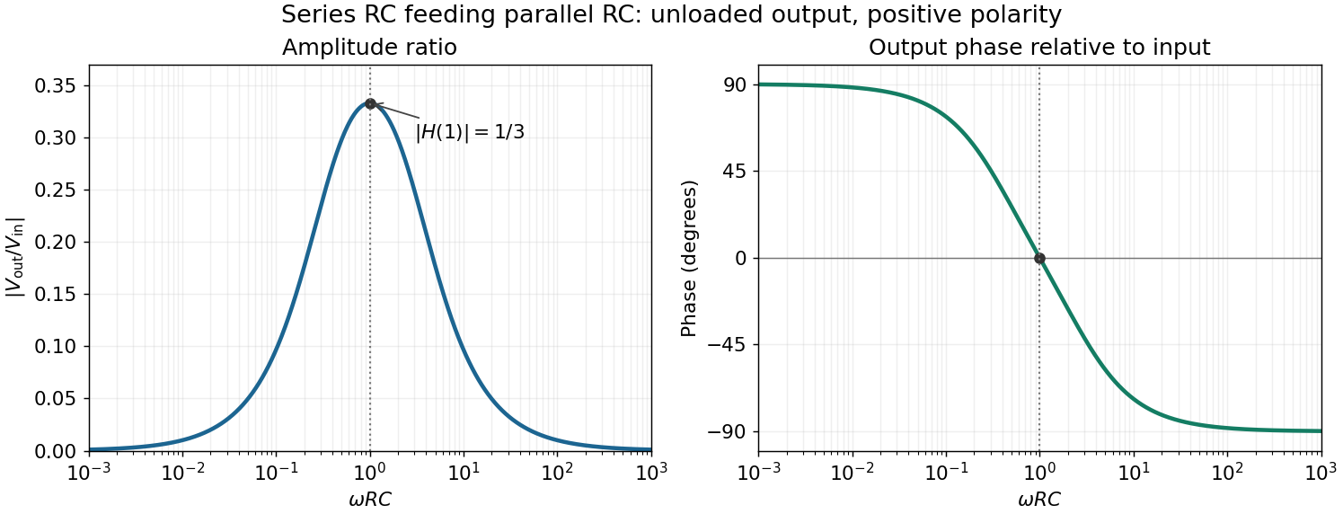
For positive angular frequency, the squared amplitude response of the series-parallel RC band-pass filter isIts denominator is minimized exactly when $w=w^{-1}$, soThis is a band-pass filter maximum produced entirely by the two RC arms; the drawn electrical circuit contains no inductor. The low- and high-frequency limits areThus the output amplitude tends to zero linearly with $\omega$ at low frequency and as $1/\omega$ at high frequency. In real time,The upper series capacitor suppresses low frequencies, while the lower shunt capacitor suppresses high frequencies.

In the chosen phasor convention, output phase minus input phase isThe real part of the denominator is positive, so this principal arctangent is continuous throughout the positive-frequency range. Below ${\omega }_0$, the output leads the input, approaching $+\pi /2$ at low frequency. Above ${\omega }_0$, it lags, approaching $-\pi /2$ at high frequency. At the maximum,The input and output are in phase there, with the positive one-third voltage ratio found above.