Local equivalence and tides. In Newtonian mechanics, inertial mass measures the response to a force, whereas passive gravitational mass couples to an imposed Newtonian gravitational field. A freely falling body obeys
The observed composition independence of free fall says that this ratio is universal. With a common choice of units it is one. This is the Newtonian content of the weak equivalence principle for test particles; it does not by itself specify all nongravitational physics.
The Einstein equivalence principle further says that local nongravitational experiments in a sufficiently small freely falling laboratory have the form predicted by special relativity, independently of the laboratory's location and motion. In such a local inertial frame, the metric tensor is locally the Minkowski metric and the Christoffel symbols vanish at the selected event. The strong equivalence principle extends the universality claim to local gravitational experiments and bodies with significant gravitational self-energy. None of these statements removes measurable tidal forces across a finite apparatus.
In an ideal small freely falling lift, a released ball initially floats relative to the cabin, because both undergo the same free fall. Two separated balls, however, need not retain their separation: they sample different parts of the gravitational field. For a point source, linearizing across a small separation gives the tidal tensor prediction
A radial separation stretches with coefficient , whereas a transverse separation is compressed with coefficient . Initially parallel velocities therefore develop relative motion even though the individual bodies experience zero proper acceleration.
The relativistic statement is geodesic deviation. With the Riemann curvature tensor convention
a connecting vector between neighboring freely falling worldlines satisfies
Here is the covariant derivative along the reference geodesic, and its four-velocity. Curvature can be nonzero where the Christoffel symbols have been made zero. In the weak, static, slow-motion limit this equation reduces to , recovering the tidal tensor above. A finite falling lift can detect gravity through these relative accelerations; local equivalence does not imply a globally uniform field.
Weak-field connection and potential. Take and the metric signature. There is an index error in the printed formula for the Christoffel symbols: its first differentiated metric component must be , not . The correctly contracted expression is
The offending term vanishes under the stipulated time independence, so this correction does not change the intended calculation. Write and treat both and its derivatives as first order. To that order , , and . A stationary metric tensor gives
For the temporal component the inverse-metric coefficient is already first order, so
For a spatial component the zeroth-order inverse metric contributes:
The time component of the approximate geodesic equation says that is constant to the retained order. In its spatial component, convert the proper time derivatives to coordinate-time derivatives and cancel :
Comparison with the Newtonian equation identifies . For an isolated source, choose the gravitational potential to tend to zero at infinity and normalize the time coordinate there, giving . Thus
The quantity is the Newtonian gravitational potential, or gravitational potential energy per unit mass, in . For a point source, . A static clock has , connecting the Newtonian limit with gravitational time dilation.
Frequency of the orbiting source. Treat the gas blob as a test particle on a timelike circular Schwarzschild geodesic, with pressure and other nongravitational forces negligible. Treat our very distant location as infinity, so the observer's own gravitational potential is negligible. These are the assumptions that make a unique answer in terms of possible.
Put and use a local static observer at the emission point as an intermediate measuring frame. The remote observer lies on the symmetry axis of the orbit. A ray arriving on that axis has zero conserved axial angular momentum, so its local direction is perpendicular to the emitter's azimuthal velocity. Bending within a meridional plane does not alter this orthogonality. The transverse relativistic Doppler effect therefore gives
where is the orbital speed measured by that local static observer. The gravitational redshift between static Schwarzschild observers then gives
A gravitational circular orbit has in the weak-field limit, so . Expanding both factors,
Solving for the emitted frequency gives
The gravitational part is and the transverse kinematic time dilation contributes another ; the absence of line-of-sight motion does not remove this second effect.
As an exact check, the local speed on a timelike circular Schwarzschild geodesic satisfies , where . Therefore the face-on frequency shift of a circular Schwarzschild source is
whose expansion agrees with the boxed answer. If the gas is supported or accelerated by pressure or magnetic stresses rather than following a geodesic, its orbital speed is not fixed by the mass and radius alone; the appropriate first-order result is instead , with supplied independently.
Doubt was reasonable if it concerned the physical cause or unlimited extrapolation of Newton's law of universal gravitation; wholesale dismissal of the quantitative evidence was harder to justify. Early eighteenth-century investigators had to distinguish the success of an inverse-square force law in explaining observations from the claim that every material body directly attracts every other one without a mediating mechanism.
The strongest case for Isaac Newton's framework was its unification of phenomena previously treated separately. Kepler's third law and nearly elliptic orbits could be connected to an inverse-square central force. Comparing terrestrial gravity with the centripetal acceleration of the Moon supported continuity between falling bodies and celestial motion. The Philosophiae Naturalis Principia Mathematica by Isaac Newton also developed treatments of interacting bodies, tides and the Earth's figure. These were substantive tests and organized a research programme capable of producing further quantitative comparisons.[ref]
There were nevertheless rational reservations. A law proportional to inferred from accessible bodies and distances did not logically establish unrestricted universality. Individual celestial predictions involved uncertain observations and approximations to difficult many-body classical mechanics. The Moon's motion and the Earth's shape were demanding tests whose successful treatment was not complete at the beginning of the century. A dissenter could question auxiliary assumptions, numerical accuracy or the inference from special cases without denying every success.
A deeper objection concerned explanation. In traditions requiring contact mechanisms, unexplained attraction across empty space appeared to reintroduce an occult quality. René Descartes's vortices supplied a mechanical alternative, though they faced their own serious dynamical difficulties. Newton himself separated a mathematically established pattern from a claimed cause of gravity; the 1713 General Scholium by Isaac Newton declined to invent an unsupported physical mechanism. Treating every criticism of action at a distance as a failure to understand evidence would therefore misrepresent the available positions.[ref]
Later confirmations cannot be counted as evidence already possessed by an early-eighteenth-century critic. Subsequent geodetic measurements, improved lunar theory and successful comet predictions helped shift the balance, but their timing matters. Nor did retaining a mechanical alternative remain equally reasonable after every failed prediction: responsible doubt required comparative assessment and willingness to revise it. The balanced conclusion is that selective, explicit scepticism about universality or cause was defensible, while the breadth of Newtonian mechanics' quantitative achievements already imposed a substantial explanatory burden on rival accounts.
Downward-from-space optical depth at wavelength is
where is the mass absorption coefficient. A nearly isothermal, hydrostatic equilibrium, compositionally well-mixed atmosphere with height-independent has and with . Thus temperature, mean molecular mass and gravity set the basic scale height. Changes in the absorber mixing ratio, pressure broadening, temperature dependence of line strengths, collision-induced absorption and departures from hydrostatic equilibrium modify it. For example if local absorption scales as in an isothermal atmosphere, .
A cold, self-gravitating region in a molecular cloud can collapse when gravity overcomes thermal, turbulent and magnetic support. Increasing central density produces a protostar, while radiation removes part of the released gravitational energy. The cloud initially carries angular momentum; material that cannot fall radially to the centre settles into a rotating protoplanetary disk. Collisions and cooling reduce random vertical motion, while angular-momentum transport allows some material to accrete and some to move outwards. Bipolar outflows and magnetic stresses can remove additional angular momentum.
The schematic sequence is . In the cool disk, grains condense and collide; settling and concentration can produce planetesimals, whose gravitational growth leads to planetary embryos. Massive cores may capture gas before the disk disperses; sufficiently massive unstable disks can also form bound condensations. Migration and interactions modify the final orbits. Radiation, accretion and outflows eventually disperse the remaining gas. Thus planet formation uses the same rotating reservoir produced by ordinary star formation, although the efficiency and final architecture are not universal and individual growth stages remain active research topics.
Neglect disk self-gravity and take around a central point mass . Its vertical gravitational acceleration is
Vertical hydrostatic equilibrium is . For a vertically isothermal ideal gas, and is independent of , giving
Here , is the isothermal sound speed squared, and is the Gaussian scale height. A different convention writing changes the quoted height by but not the physics.
At latitude , the Earth's angular velocity in east–north–up coordinates is . Assume a small horizontal patch, constant , negligible vertical velocity, and a vertical constraint balancing effective gravity. Absorb the steady centrifugal force into that effective gravity. With and physical horizontal force per unit mass , the Coriolis force gives
Large-scale atmospheric and oceanic flows deflect to their right in the northern hemisphere and left in the southern hemisphere; their balance with a horizontal pressure gradient produces geostrophic flow. A Foucault pendulum has an oscillation plane that precesses relative to the ground at angular rate . Both effects vanish at the equator within this horizontal approximation.
The collision cross section in the incoming impact-parameter plane is
Without gravity it is only , so gravitational focusing increases the cross-section by . Trajectories that would miss geometrically can be bent into contact, especially for slow relative encounters. Gravity does not itself guarantee sticking: the following accretion estimate assumes collisions agglomerate rather than fragment, rebound or erode the target.
A uniform incoming projectile mass density has mass flux , so
The formula counts mass swept per unit time and assumes an adequate continuing projectile supply, the stated speed, and negligible many-body or stellar-tidal modification of the two-body cross-section.
Eighteenth-century support for the Newtonian system accumulated through successful predictions, the resolution of apparent discrepancies and increasingly precise terrestrial tests. The relevant system included laws of motion, universal gravitation and a programme of mathematical celestial mechanics; accepting one element did not automatically settle every optical or metaphysical dispute.
Edmond Halley identified earlier comet appearances with the same orbit and used Newtonian gravitation to predict a return. Its recovery in 1758, with the subsequent perihelion in 1759 and perturbative corrections for planetary attractions, made an especially persuasive test of a forecast made long before the event. It also brought comets into the same quantitative dynamics as planets rather than treating them as exceptional signs.[ref]
Geodetic expeditions compared meridian arcs at different latitudes. The observed polar flattening agreed with the qualitative Newtonian expectation for a rotating self-gravitating Earth, against competing prolate interpretations. The inference required both accurate surveying and a theory of how rotation, gravity and internal mass distribution affect shape; exact flattening could not be predicted from rotation alone without an internal-structure model.[ref]
Lunar and planetary perturbation theory provided a sustained, more demanding test than unperturbed Keplerian ellipses. Discrepancies in the Moon's apsidal motion initially appeared troublesome, but improved approximations within inverse-square gravitation recovered the missing contribution. Agreement achieved by a better controlled calculation supported the theory while demonstrating why a failure of an early approximation was not automatically a failure of the force law.
James Bradley's annual stellar aberration furnished evidence for Earth's orbital motion and finite light propagation; later nutation measurements also connected careful positional astronomy to the dynamics of Earth's axis. Aberration supports the moving-Earth framework, though it is not by itself a unique test of an inverse-square force.[ref]
Finally, Henry Cavendish's torsion-balance experiment in 1798 measured attraction between laboratory masses and inferred Earth's mean density. It extended gravitation from celestial fitting to a quantitatively controlled terrestrial attraction; describing the original aim as determining Earth's density is historically more accurate than saying he set out to measure a modern separately defined . Together these tests supplied converging support across scales. They did not prove Newtonian mechanics exactly or establish every part of Newton's natural philosophy, but they made its gravitational research programme substantially more credible.
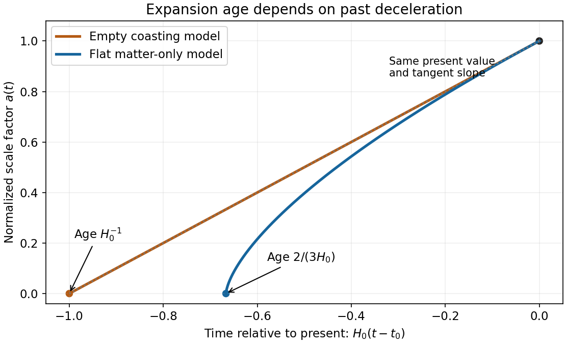
With zero curvature and no cosmological constant, the present normalization requires . Thus , and choosing the big bang as gives
For an empty expanding model, and the curvature must be negative. The equation becomes , giving
The latter is the Milne slicing of flat spacetime; its zero-scale-factor origin is not a matter-density curvature singularity. In the matter model, gravity decelerates expansion, so the earlier slope was greater than the present slope and the same present size was reached in less time. With the stipulated , the two model ages are approximately and Gyr.
Figure 1.
Equal present expansion rates give different ages when matter decelerates expansion
. Both normalized scale factors reach one at the present and have the same slope there. The matter-only curve begins two thirds of a Hubble time before the present; the empty coasting curve begins one Hubble time before it. Details.
The radiation pressure at a photospheric temperature near K is only about Pa. For an illustrative photospheric gas density and mean molecular weight near , the ideal gas pressure is about Pa. Thus gas pressure dominates those outer layers by many orders of magnitude. Both the temperature and density are needed: low temperature alone is not a complete comparison.
For homologous stars, hydrostatic and ideal-gas estimates give and . Therefore
with a structural coefficient independent of mass only under the homology assumption. As mass rises, radiation becomes increasingly important. A rough solar interior normalization of - suggests equality after a mass increase by tens, while realistic radiation-dominated structure and composition shift the scale; stars of order are a useful estimate for strong radiation support. The very small photospheric ratio must not be used as a universal normalization for their whole interiors.
Radiation also transfers outward momentum. Comparing radiative acceleration with gravity gives the Eddington luminosity
Near this scale, radiatively driven winds and envelope instabilities can remove matter or impede further accretion. Opacity, composition, rotation, mass loss and formation history affect the limiting stellar mass. The Eddington condition is a luminosity-to-mass constraint, not a unique composition-independent maximum stellar mass.
Hydrostatic equilibrium means that the local pressure gradient balances gravity, with no large acceleration or strength-supported departure from that balance. In a spherical planet,
Here is the enclosed mass, not a constant total mass at every interior radius. If composition is uniform and the radial thermodynamic path is adiabatic, the relevant bulk modulus is . The chain rule then gives the Adams-Williamson relation
A phase transition or composition jump must be treated separately; its density change is not obtained by integrating one smooth homogeneous-adiabatic equation through it.
The seismic parameter is
The shear modulus measures resistance to shear deformation. Solids with transmit shear waves; an ideal fluid has zero static shear modulus, so it cannot carry a bulk S wave, while compressional P waves can still propagate through its nonzero bulk modulus.
Limitations include uncertain seismic coverage, temperature and composition tradeoffs, nonadiabatic boundary layers, phase changes, lateral heterogeneity, rotation and finite material strength. Small asteroids and comet nuclei commonly retain irregular shapes because their self-gravity is too weak to overcome strength and impact history; a few larger bodies, such as Ceres, are much closer to global hydrostatic figures. A spherical shape alone is not a complete proof of present hydrostatic equilibrium.
Two complementary remote constraints are precise spacecraft tracking, which measures gravitational harmonics and constrains mass distribution when combined with shape and rotation; and tidal or rotational measurements, such as Love numbers, librations and spin precession, which constrain deformability, moment of inertia and possible fluid layers. Magnetic induction measurements in a time-varying external field can provide an additional conductivity constraint, but are not a unique density inversion.
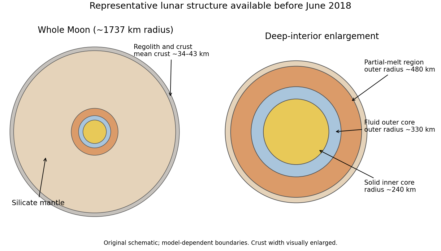
For the June 2018 lunar picture, start with a regolith and fractured crust, a largely anorthositic crust tens of kilometres thick, a silicate mantle, a deep partially molten region and a small iron-rich core. GRAIL and Apollo-based models gave a global mean crustal thickness around - km.[ref] A representative seismic model has a partial-melt boundary near radius km, a liquid outer-core boundary near km and a solid inner-core radius near km; these are model-dependent radii from the centre, not depths below the surface.[ref]
Figure 1.
A representative pre-June-2018 lunar interior model
. An original schematic cross-section labels the crust, silicate mantle, deep partial-melt region, fluid outer core and solid inner core. Approximate central layer radii are 480, 330 and 240 kilometres; the thin crust is shown with a visually enlarged width and all boundaries are model dependent. Details.
The long-running Apollo network had only four principal stations on the near side, with poor global coverage and strong scattering in the fractured near-surface material. Far-side structure and weak deep reflected phases were therefore difficult to constrain. The historical date matters: the answer does not import later Mars seismology or later lunar-core refinements into the 2018 premise.
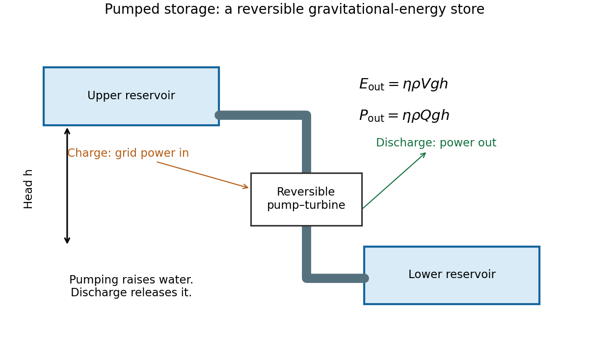
A pumped-storage plant moves water uphill using electrical power, then returns it through a turbine and generator when electricity is needed. The upper and lower reservoirs set the usable volume and head; pumps, penstocks, valves and reversible pump-turbines set the power and flow. The plant stores energy rather than generating net energy over a cycle.
Figure 1.
Gravitational storage separates reservoir energy capacity from pump and turbine power
. An original functional diagram shows an upper and a lower reservoir connected through a penstock and reversible pump-turbine. Charging uses grid electricity to lift water; discharge returns gravitational potential energy through the generator. Details.
For constant head, the gravitational energy is . With the stated generation efficiency,
At GW, gives
Head variation, dead volume and hydraulic losses beyond the stipulated efficiency have been neglected.
To deliver kWh with the same head and efficiency needs of water, roughly a m cube, together with a m elevation difference and a lower reservoir. At a m head it would need about . This contrasts with the small fuel volume: the useful energy density of lifted water depends on its external head, not its chemical composition.
Pumped storage offers long service life, fast dispatch, substantial power, and separate choices of storage volume and turbine rating. Its drawbacks include geographic constraints, construction cost and time, ecological impacts, evaporation and water requirements, plus round-trip losses. The quoted generation efficiency alone is not the round-trip efficiency because pumping also consumes more than the stored potential energy.
The rock cylinder has mass and rises through . Equating its useful energy to the reservoir result cancels the common efficiency and gravity:
Its height is about m and its lift about m, ignoring buoyancy as instructed. Stored energy scales as , excavated volume roughly as , and lined area as . If excavation dominates cost, cost per unit stored energy decreases approximately as . Seals, increasing pressure, geology, leakage, supporting structure and power equipment can change that scaling; a volume law is not a complete cost model.
Differentiation gives
The angles and are cyclic, so their canonical momenta are conserved. The Lagrangian is autonomous, so the total energy is also conserved. The momentum is not generally constant because gravity and the angular kinetic terms depend on .
The relevant comparison is between gravity and surface tension. With the mass density difference , the Bond number and capillary length are
Thus the drop is small compared with the capillary length; hydrostatic pressure variations only weakly perturb its shape. The Young–Laplace equation then gives approximately constant interfacial mean curvature, and an axisymmetric drop on a uniform flat substrate is a spherical cap. The substrate selects the contact angle, measured through the water.
Write for the radius of the generating sphere, for the contact-circle radius, and for the apex height. Elementary trigonometric identities give
Taking the stated droplet radius to mean its radius of curvature, , gives
There is no diagram or explicit radius convention in the original PDF. If instead denotes the contact-circle radius, the answer is . If it denotes the radius of an equal-volume free sphere, use the volume of a spherical cap, , to obtain . The spherical cap approximation is justified in all three conventions; a unique numerical height requires specifying which radius is meant.
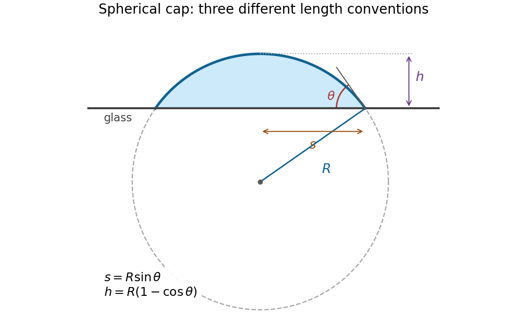
Figure 1. . Original cross-section distinguishing the generating-sphere radius , contact-circle radius , and height . The dashed part of the generating circle lies below the substrate. Details.
Suppress hats for this calculation. Transverse pressure uniformity and zero surface pressure give throughout the film. Thus . Integrating twice, using and , gives
The flux is . Integrate continuity across the layer and apply the wall and kinematic conditions to obtain . Restoring hats yields
The cubic flux contains downward gravity-driven transport and upward wall entrainment.
For positive surface tension the threshold is even in , tends to infinity as and as , and has its two equal minima at
Minimizing for gives
Thus the initial state has some exponentially growing mode exactly when . If , the unstable band is
Gravity suppresses long wavelengths and surface tension suppresses short ones; intermediate wavelengths become unstable when the shear is large enough.
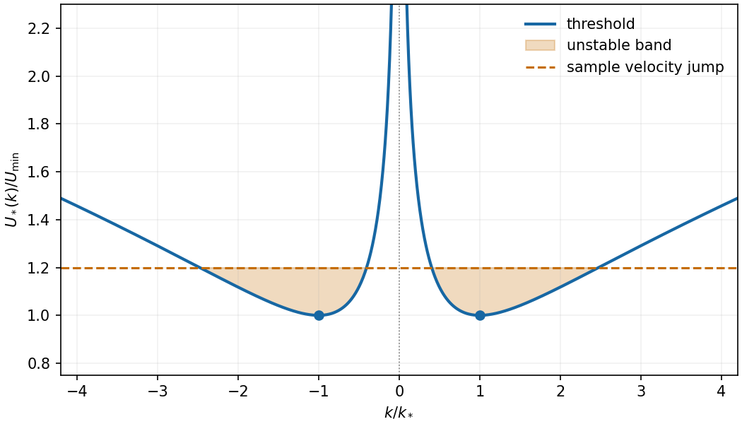
Figure 1.
Even instability threshold with minima at the gravity-capillary balance; the sample shear destabilizes the shaded intermediate bands
. Details.
The four dimensional equations express mass conservation, momentum balance with pressure, gravity and viscous stress, heat advection and conduction, and a linear thermal-expansion equation of state. For heating from below, suitable plate conditions are and at , and , at . No slip and thermal insulation on the sidewall provide one suitable lateral completion; prescribed lateral temperatures would be another specified thermal setup.
Let be thermal diffusivity and kinematic viscosity. Use , , and as length, time, velocity and temperature scales. Subtract the static reference pressure with and scale its remainder by . Then
Density becomes . Substitution and division by the corresponding diffusion/viscous scales give
In the Boussinesq small-density-contrast limit retain buoyancy while neglecting the other factors. At infinite Prandtl number, after any fast initial adjustment, the equations are
The velocity is instantaneously constrained by a viscous elliptic balance; the temperature still evolves.
Take the divergence of the vector Poisson equation. Derivatives commute, and divergence of a curl is zero, so . Its boundary value is zero, hence the maximum principle gives throughout . The vector identity now gives , or
The layer domain is simply connected because its horizontal section is simply connected. For a curl-free field on such a domain, define as its line integral from a fixed base point to . Contractibility of loops and Stokes theorem make the integral path independent, and differentiation gives its gradient equal to the field. Thus .
Incompressibility then gives , while the prescribed normal curl gives . Green's identity yields
Hence is constant on the connected domain and . The extra condition belongs to the stated potential boundary problem; the reconstruction argument above uses the divergence and normal-curl conditions. On a multiply connected domain a curl-free field need not be a globally single-valued gradient.
Finally . Taking the curl of the infinite-Prandtl momentum balance and using gives
The derivation is an instance of velocity reconstruction from a mixed-boundary vector Poisson problem.
Choose vertically upward. Let be the gas-occupied part of a pipe cross-section, of area . Define the phase mean mass density, mass-weighted velocity, second moment of velocity, and phase mean pressure by
The void fraction is a volume fraction, not a mass fraction. The gas momentum in a slice of length is ; its advected momentum flux is . The two end pressures give the net force . Include every other vertical force on the gas, including interfacial forces, in . Newton's second law for this fixed slice, followed by division by , therefore gives
This is a cross-section averaged phase momentum balance. In particular, mass weighting makes the momentum and its flux exact averages; one must not replace by without an additional closure. With liquid mean velocity , constant liquid mass density , and liquid second moment , the same calculation gives
With the common pressure , the specified pressure contributions to cancel the phase-fraction derivatives from the product rule. The remaining pressure forces per unit mixture volume are and .
Assume that the bubbles at a given height have the stated radius . Their number per unit mixture volume is . The drag force on a rising bubble opposes its relative velocity, so multiplication of the single-bubble law by gives the signed magnitude
Gravity acts downward; the drag force on the liquid is the opposite of that on the gas. With no wall force,
A bubble retains its mass in the absence of transfer between phases. Consequently and
For clarity suppress bars on in the steady calculation. On a macroscopic variation length , gas inertia per unit volume scales like , whereas the quadratic drag force scales like . Their ratio is . Thus , together with the scale separation inherent in this averaging model, justifies the leading-order neglect of gas inertia. Small reference density alone does not justify it in an arbitrarily short or strongly compressed region. Neglect gas weight at the same order, with the liquid fraction not vanishing. For a stationary liquid, summing the two momentum equations gives
The leading gas balance is . Substitution of the bubble-radius law yields
The gas continuity equation, with constant pipe area and no mass exchange, is . Hence the steady gas mass flux is constant. For the pressure equation selects , and
Evaluate the latter constant at a reference point , and divide. The terminal-drift density law for compressible bubbles is
The exponent comes from combining mass conservation with the density dependence of bubble radius; no gas equation of state was needed.
Use an asymptotic expansion at fixed , evaluating the boundary conditions at the instantaneous . At leading order, the downslope equation gives . The wall condition and the surface condition imply
Here denotes the total leading velocity, to distinguish it from the dimensional scale . The continuity equation and wall impermeability then give
The transverse momentum equation gives . The normal stress condition therefore yields
The leading volume flux per unit width is . Consequently mass conservation gives . This relation eliminates inside the first inertial correction:
Set . The downslope equation and boundary conditions are
Two integrations give
The pressure correction is not needed for this calculation because its downslope pressure gradient enters only at .
Integrating the total velocity across the film gives
Indeed the three inertial polynomial terms integrate to . Integrating the continuity equation and using the kinematic boundary condition gives . Hence the Benney equation is
Normal gravity smooths height variations on the upper side of the slope, while the inertial correction can amplify them. Surface tension suppresses sufficiently short wavelengths.
For an inverted falling film, keep directed from the solid into the liquid. The downslope component of gravity is unchanged, but its normal component is now positive. Thus the hydrostatic pressure changes from to . The resulting Benney equation is
Only the normal-gravity contribution changes sign; the surface tension and inertial contributions retain their signs.