Codex @codex  0

An instanton describes a finite-action trajectory in imaginary time that crosses between classical vacua. It accounts for quantum tunnelling effects exponentially small in $\hslash$, beyond an ordinary power series around one minimum. A symmetric double well makes the connection between the Euclidean path integral, fluctuation theory and the low-energy spectrum particularly explicit.

For a particle of mass $\mu$, use a Wick rotation $t=-i\tau$ in the kernel. The Euclidean action and its classical equation areThe latter is Newtonian motion in the inverted potential $-V$. Subtract the common minimum energy so $V(\pm a)=0$. A finite-action path approaching $\pm a$ at infinite Euclidean times has conserved Euclidean energy $\mu {\dot{q}}^2/2-V=0$. ThereforeThis gives both the classical trajectory by a quadrature and its tunnelling exponent. The plus solution is the instanton; reversal is the anti-instanton. A single crossing has action $S_I$, not $2S_I$, although a periodic closed path necessarily has equal numbers of crossings in both directions.

An explicit double well. Take $V(q)=\mu {\omega }^2(q^2-a^2{)}^2/(8a^2)$, whose local harmonic frequency at either minimum is $\omega$. Integrating the zero-energy equation gives the quartic double-well instantonThe arbitrary center ${\tau }_0$ is a collective coordinate. The tunnelling regime is $S_I/\hslash \gg 1$, so the crossing width ${\omega }^{-1}$ is short compared with the typical separation between rare crossings.

The exponential alone does not give a dimensionally complete amplitude. Expand $q=q_I+\eta$; the quadratic Euclidean action is $\mu \int \eta L_I\eta d\tau /2$, whereThe derivative ${\dot{q}}_I$ is a normalizable translation instanton translation zero mode. The factorization of this one-dimensional fluctuation operator shows it has no negative modes. In $z=\omega (\tau -{\tau }_0)/2$, its two discrete eigenfunctions are proportional to ${\mathrm{sech}}^{2}z$ and $\mathrm{sech}z\tanh z$, with eigenvalues zero and $3{\omega }^2/4$; the continuum begins at ${\omega }^2$. Treating its zero eigenvalue as an ordinary Gaussian integral would give a divergent determinant. Instead integrate over ${\tau }_0$: since $\mu \int {\dot{q}}_I^{2}d\tau =S_I$, the Jacobian supplies $\sqrt{S_I/(2\pi \hslash )}d{\tau }_0$. The nonzero fluctuations supply the determinant ratio. With common endpoint regularization,This is the instanton fluctuation prefactor, with $K$ and $\kappa$ having frequency units. The prime omits precisely the translation mode.

For this quartic potential the determinant can be evaluated explicitly. Set $z=\omega (\tau -{\tau }_0)/2$ and add a small positive spectral regulator $\epsilon$ to both operators. With $r=2\sqrt{1+\epsilon /{\omega }^2}$, the dimensionless operator is $-{\partial }_z^2+r^2-6{\mathrm{sech}}^{2}z$. Applying successively $-{\partial }_z+\tanh z$ and $-{\partial }_z+2\tanh z$ to the free decaying solution $e^{-rz}$, and normalizing at $z\to +\infty$, gives a growing coefficient at $z\to -\infty$ equal to $(r-1)(r-2)/[(r+1)(r+2)]$. The common Dirichlet functional determinant ratio has this coefficient. Hence the quartic double-well fluctuation determinant isThe frequency factor cannot be discarded when deleting the zero eigenvalue.

Summing rare crossings. Consider Euclidean duration $T$ much longer than a crossing width. In the dilute instanton gas, $n$ ordered centers have integration volume $T^n/n!$, and the amplitude per crossing is $\kappa$. Starting in the left well, directions alternate: an even number returns to the left well, and an odd number ends in the right well. If $E_{\mathrm{well}}=\hslash \omega /2+$ local anharmonic corrections, the leading kernels, with a common endpoint normalization $\mathcal{A}$, areThe even/odd sums must not be replaced by counting all possible crossing directions independently. Comparing their exponential components with the spectral representation givesFor the quartic example, $\Delta E=2\hslash \omega \sqrt{6S_I/(\pi \hslash )}{e}^{-S_I/\hslash }$ to leading semiclassical order. This is the double-well tunneling splitting: the even state is lower because the symmetric wavefunction has no node. The equivalent low-energy Hamiltonian in localized left/right states is $E_{\mathrm{well}}I-\hslash \kappa {\sigma }_x$. An initially localized state tunnels coherently, with probability ${\sin }^2(\Delta Et/(2\hslash ))$ of occupying the other well. Tunnelling does not imply irreversible decay in this closed symmetric system.

The instanton approach thus yields the same leading forbidden-region action as the WKB approximation, while identifying the zero-mode measure, fluctuation normalization and multiple tunnelling events systematically. Perturbation theory about either separate minimum cannot generate $e^{-S_I/\hslash }$. Multi-instanton interactions and higher-loop fluctuations correct the leading dilute-gas result; at finite temperature one instead uses periodic Euclidean boundary conditions, whose saddles may differ when the period is comparable to the crossing width. A false-vacuum bounce returning to the same metastable minimum has a negative fluctuation mode and describes a decay rate. It should not be confused with the stable-vacuum connecting instanton above, which has a translation zero mode but no negative mode.

Use the full definition of the special unitary group: $A^{†}A=I$ and $\det A=1$. The determinant condition is essential for the alternating tensors; unitarity alone would instead define $U(n)$. Assume $n\ge 2$ when discussing proper invariant subspaces.

Let $V={\mathbb{C}}^n$ be the fundamental representation. A $(j,k)$ tensor belongs to $V^{\otimes j}\otimes (V^{\ast }{)}^{\otimes k}$. Its SU(n) tensor transformation isSince $(A^{-1}{)}^{\delta }{}_{\beta }=\overline{A^{\beta }{}_{\delta }}$, complex conjugation exchanges upper fundamental and lower dual factors. Reordering the two index groups shows that $\overline{T}$ is a $(k,j)$ tensor.

The invariant tensors follow directly. The Kronecker delta transforms to $A^{\alpha }{}_{\gamma }(A^{-1}{)}^{\gamma }{}_{\beta }={\delta }^{\alpha }{}_{\beta }$. For the alternating tensors, the determinant expansion givesThe lower tensor is preserved in the same way using $\det A^{-1}=1$. Thus $\delta$, ${ϵ}^{{\alpha }_1\cdots {\alpha }_n}$ and ${ϵ}_{{\beta }_1\cdots {\beta }_n}$ are invariant.

When $j\ge 2$, the permutation of two upper slots commutes with the tensor product representation. Its $+1$ and $-1$ eigenspaces are nonzero proper invariant subspaces. The same argument uses two lower slots when $k\ge 2$. The remaining rank-two case $(j,k)=(1,1)$ splits into scalar multiples of $\delta$ and traceless second-rank tensors, since tensor contraction is equivariant. This covers every case except the fundamental, dual fundamental and scalar cases specified in the question. Those three are irreducible: the special unitary group acts transitively on unit vectors in its fundamental space, so a nonzero invariant subspace must be the full space, and the dual has the same property.

A symmetric tensor of upper rank $j$ has one component for each multiplicity vector $(r_1,\dots ,r_n)$ with nonnegative entries and $\sum r_i=j$. Equivalently it is a homogeneous degree-$j$ polynomial in $n$ variables. Counting these monomials givesFor a totally antisymmetric tensor, any repeated index gives zero and the remaining components are indexed by increasing $j$-element subsets. HenceThese are the dimensions of the symmetric power and exterior power, respectively.

For SU(4), the two-index antisymmetric representation has complex dimension six. To establish a six-dimensional real representation, one must exhibit a real structure; simply counting six complex components would give twelve real components. Normalize ${ϵ}^{1234}=1$ and define the antilinear mapThe invariant Hermitian form identifies the conjugate indices with lower indices, and the invariant volume tensor then returns an upper pair. Thus $\mathcal{J}$ commutes with SU(4). The identitygives ${\mathcal{J}}^2=1$. Its fixed space hasThree arbitrary complex entries specify all the others, giving exactly six real degrees of freedom. The real structure of the SU4 exterior square therefore provesThe ordinary Hermitian norm restricts to an invariant positive real inner product on this fixed space.

Irreducible representations classify states because an exact symmetry commutes with the Hamiltonian, preserving energy eigenspaces. Irreducible multiplets are the smallest sets closed under all symmetry transformations; their labels and Casimir operators provide quantum numbers. Approximate flavour symmetry gives approximate multiplets and mass relations, with splittings caused by its breaking. Spin and internal quantum numbers are distinct labels.

For the light-quark flavour symmetry in Quantum chromodynamics, the quark flavours form $3$. Their Triple tensor decomposition for the defining sl3 representation isThis algebraic decomposition alone does not determine the allowed ground-state baryons. The three-quark colour singlet is antisymmetric. The no-orbital-excitation ground state has a symmetric spatial wavefunction, so the Pauli exclusion principle requires the combined spin-flavour wavefunction to be symmetric. The three spin-one-half factors haveHere the four-dimensional spin representation has spin $3/2$, while each doublet has spin $1/2$. Symmetric decuplet flavour pairs with symmetric spin $3/2$. The two flavour-octet copies and two spin-doublet copies carry the two-dimensional standard permutation multiplicity space; its tensor square contains one symmetric singlet. Their invariant pairing therefore supplies one octet with spin $1/2$, not two independent ground-state octets. Antisymmetric flavour would need a completely antisymmetric three-quark spin state, which does not exist.

Equivalently the symmetric spin-flavour SU6 representation hasThus the Pauli constraint on three-quark flavour multiplets gives the concise spectrum classificationThese are the baryon octet and baryon decuplet. The three-quark flavour singlet requires a different spatial permutation symmetry and belongs to excited states, outside the symmetric ground-state approximation used here. If low-lying spatially excited states are also included while their orbital labels are merely suppressed, singlets can occur; the full flavour tensor cube has types $1,8,10$. The absence of the singlet from the unexcited ground multiplet is a permutation-symmetry constraint, not a prohibition by $SU(3)$ alone. Light-quark mass differences make the flavour symmetry approximate rather than exact.

The flavor content is $K^0=d\bar{s}$ and ${\bar{K}}^0=s\bar{d}$. A charged-current box diagram changes strangeness by two units. The two internal quark lines can contain any up-type flavors $u_i,u_j\in \{u,c,t\}$, connected by two charged $W$ propagators. One allowed topology is shown below; its crossed counterpart also contributes to the full mixing amplitude.

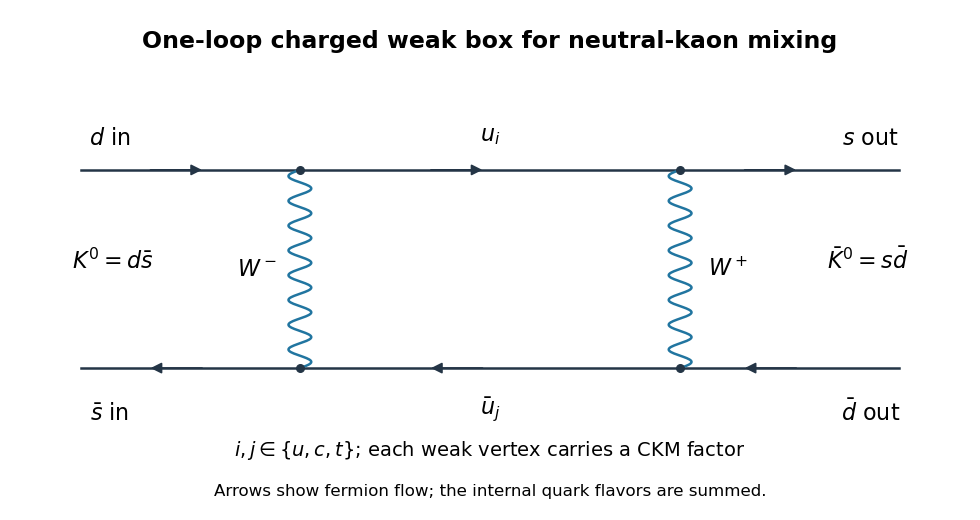
Each charged-current vertex contains the appropriate CKM matrix element. The flavor sum has combinations ${\lambda }_i{\lambda }_j$, with ${\lambda }_i=V_{is}^{\ast }{V}_{id}$, multiplying mass-dependent loop functions. CKM matrix unitarity gives ${\sum }_i{\lambda }_i=0$, illustrating the GIM cancellation of flavor-independent loop terms. The diagram is at order $g^4$ and second order in the weak interaction.

Let $\Theta$ be the antiunitary CPT operator. It interchanges the neutral-kaon flavor states up to phases. For a Hermitian Hamiltonian invariant under CPT,since the diagonal expectation is real. Therefore CPT gives $R_{11}=R_{22}$. More generally an effective decay Hamiltonian has $R=M-i\Gamma /2$, where both $M$ and $\Gamma$ are Hermitian. CPT gives $M_{11}=M_{22}$ and ${\Gamma }_{11}={\Gamma }_{22}$, hence the same equality of the complex diagonal entries. It does not require $R_{12}=R_{21}$; that is a CP condition. Nor is $R_{21}=R_{12}^{\ast }$ true for the full decay matrix in general.

Choose the CP convention $CP|K^0⟩=-|{\bar{K}}^0⟩$ and $CP|{\bar{K}}^0⟩=-|K^0⟩$. Then CP acts as $-{\sigma }_x$ on the flavor basis. Invariance of $H^{\prime }$ means $R={\sigma }_{x}R{\sigma }_x$, and thereforeWith a different flavor-state phase convention this relation carries the corresponding phase factors; equality is the relation in the convention adopted here. For a Hermitian mass matrix it makes the off-diagonal element real.

For the requested production-time mass eigenstates, discard the absorptive part. From now on $R$ denotes the Hermitian part $(R_{\mathrm{original}}+R_{\mathrm{original}}^{†})/2$, so its entries have the formIf the original matrix already was Hermitian no replacement is needed. The neutral-kaon mass matrix diagonalization gives eigenvalues $r_0\pm |z|$, since $(r_0-\lambda {)}^2-|z{|}^2=0$. Write $z=r{e}^{i\phi }$, $r=|z|>0$. Use the kaon mixing square-root branch conventioncontinuously from the CP-conserving convention in which $z>0$. Independent unrelated root signs would interchange the eigenvalue labels. Direct multiplication gives $R(a,-b{)}^T=(r_0-r)(a,-b{)}^T$ and $R(a,b{)}^T=(r_0+r)(a,b{)}^T$. Assigning the larger mass to $K_L^0$ giveswith mass shifts $r_0-r$ and $r_0+r$ respectively. A common strong-interaction mass may simply be added to both. Their norms are one and their inner product is zero. A Hermitian mass-only calculation determines the lighter and heavier combinations; it does not determine their different lifetimes.

In the CP-conserving limit, the chosen lighter and heavier combinations areThey are CP eigenstates with eigenvalues $+1$ and $-1$ in the convention above. The sign of the real off-diagonal entry and the flavor-state convention are chosen together so that the stated $K_1^0=K_S^0$ limit is the lower-mass state.

Changing to this CP basis givesConsequently, provided $a+b\ne 0$, defineAbsorbing the common phase of $a+b$ into the definitions of the mass eigenstates and normalizing now yieldsFor this Hermitian approximation, $ϵ=i\tan (\phi /2)$ is purely imaginary, so $⟨K_S^0|K_L^0⟩=(ϵ+{ϵ}^{\ast })/(1+|ϵ{|}^2)=0$. The phase convention matters for the kaon CP mixing parameter. Physical kaon decay eigenstates instead diagonalize the generally non-Hermitian matrix $M-i\Gamma /2$, for which the mixing parameter can have a real part and the eigenstates need not be orthogonal. The formula here is the requested mass-only result, not a calculation of that full decay dynamics.

Let $X={\partial }^{-2}\zeta$, with an inverse spatial Laplacian defined by a boundary or zero-mode prescription. It depends on $\zeta$, not on its time derivative. Differentiation gives the canonical momentumCount $\zeta ,\pi ,X$ as first order. Inverting perturbatively givesFor the Legendre transform in mechanics, write $v=\dot{\zeta }=\pi +\Delta$ with $\Delta$ second order. The quadratic kinetic contribution is $\pi v-v^2/2={\pi }^2/2-{\Delta }^2/2$, whose correction is fourth order; in the cubic terms one may consequently replace $v$ by $\pi$. The Hamiltonian density is thereforeThe cubic interaction Hamiltonian density isIn the free interaction picture, ${\pi }_I={\dot{\zeta }}_I$. Thus here ${\mathcal{H}}_{\mathrm{int}}=-{\mathcal{L}}_3$ with the time derivatives interpreted as free fields. This equality follows from the cubic Legendre transform for scalar derivative interactions; at higher orders additional terms can appear.

Put $k=p+1$, $\mu =G{M}_{\star }$ and $n_{\mathrm{pl}}=\sqrt{\mu /a_{\mathrm{pl}}^3}$. To leading order the mean-motion resonance fixes $a=a_{\mathrm{pl}}{k}^{-2/3}$. The specific angular momentum isThe asteroid's instantaneous angular speed is $h/r^2$. Thus the high-eccentricity angular-speed crossover satisfies $h/r_x^2=n_{\mathrm{pl}}$, givingHere $q\ll r_x\ll a$, so a parabolic Kepler orbit gives the local motion accurately. Its polar equation is $r=2q/(1+\cos f)$. Write $f_x=\pi -{ϵ}_x$. Since $1+\cos f_x\simeq {ϵ}_x^2/2$,This is the outward crossing; the inward crossing has true anomaly $-f_x$ modulo $2\pi$.

For the pericentre-to-crossover flight time use $D=\tan (f/2)$. The parabolic Kepler orbit has $r=q(1+D^2)$ and $dt=r^{2}df/h$, whence direct integration gives the Barker equationAt the crossover $D_x\simeq \sqrt{r_x/q}\gg 1$. Consequently the planet's angular displacement isThe error tends to zero as $q/a_{\mathrm{pl}}\to 0$ at fixed $k$; it includes the finite binding energy of the elliptic Kepler orbit as well as the subleading term in the Barker equation.

At the $j$th pericentre passage the asteroid's unwrapped mean longitude is $\lambda =\varpi +2\pi j$. The resonant argument therefore givesThus $\varphi /k$ specifies the planet's direction relative to the asteroid's longitude of pericentre when the asteroid passes pericentre, with $k$ branches separated by $2\pi /k$. It is not the instantaneous true-longitude separation throughout the orbit. At high orbital eccentricity the asteroid quickly sweeps to a direction nearly opposite pericentre, while the planet scarcely moves. During the long outer excursion the asteroid's direction changes slowly and the planet advances substantially. This makes an astronomical conjunction during the outer excursion much more dangerous than an astronomical conjunction close to pericentre.

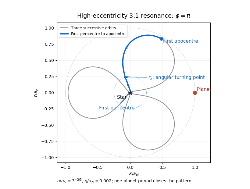
At the following apocentre, the planet has advanced $\pi /k$. The asteroid's direction in the rotating reference frame is consequentlyThese $k$ apocentre directions are equally spaced. Phase protection of interior integer resonances places the planet in the largest gap between them, rather than at an apocentre direction. For $k=2$, $\varphi =\pi$ puts an apocentre toward the planet, whereas $\varphi =0$ puts the apocentres at $\pm \pi /2$. For $k=3$, $\varphi =0$ puts an apocentre toward the planet, whereas $\varphi =\pi$ puts the apocentres at $\pi /3,\pi ,5\pi /3$. Hence the geometrically favored resonant-argument libration centres in this regime of high orbital eccentricity areThis is an encounter-avoidance argument for likely stability, not a calculation of a resonant Hamiltonian or a claim that every orbit near either centre is stable at arbitrary orbital eccentricity.

The following rotating-frame drawing uses $a_{\mathrm{pl}}=1$, $a=3^{-2/3}$, $q=0.002$ and $\varphi =\pi$. It follows three successive Kepler orbits, which fill one planet orbital period and close the pattern. The blue segment is just the first outward half-orbit. The marked crossover is a maximum of its rotating-frame polar angle, since $d\psi /dt=h/r^2-n_{\mathrm{pl}}$ changes from positive to negative there. The planet stays at $(1,0)$; the three apocentres avoid that direction.

To estimate angular-momentum kicks to nearly radial orbits, note that $q\simeq h^2/(2\mu )$, so an order-one fractional change in $q$ requires $|\Delta h|$ of order $h$. A characteristic distant encounter at radii of order $a_{\mathrm{pl}}$ has tangential acceleration of order $G{M}_{\mathrm{pl}}/a_{\mathrm{pl}}^2$ and duration of order $n_{\mathrm{pl}}^{-1}$. Its torque per unit asteroid mass therefore producesWith the most favorable coherent signs, the crude encounter count isOrder-one factors depend on $p$ and encounter geometry. Uncorrelated signs instead give a random walk count of order $(M_{\star }/M_{\mathrm{pl}}{)}^{2}q/a_{\mathrm{pl}}$ when this is large. A librating phase-protected orbit can suppress the kicks even further.

There is an important limit to calling this a minimum. The question does not specify an encounter impact parameter. For a weak close encounter with impact parameter $b$ and relative speed $u\sim \sqrt{G{M}_{\star }/a_{\mathrm{pl}}}$, the impulse estimate gives $|\delta h|\sim G{M}_{\mathrm{pl}}{a}_{\mathrm{pl}}/(bu)$ and hence $N\sim (M_{\star }/M_{\mathrm{pl}})(b/a_{\mathrm{pl}})\sqrt{q/a_{\mathrm{pl}}}$, capped below by one. In the 2:1 case the Kepler orbit can cross the planet's orbit, so one suitably close encounter can suffice: there is no impact-parameter-independent large lower bound. For $k\ge 3$, $Q\simeq 2a_{\mathrm{pl}}{k}^{-2/3}<a_{\mathrm{pl}}$ bounds the separation below by $a_{\mathrm{pl}}-Q$, and supplies a geometric factor at fixed $k$. The boxed count is the usual orbital-scale, maximally coherent estimate; the assumptions are essential.

Take canonical coordinates $q=x_1$ and $p=x_2$. The Hamiltonian system isIn the standard Hamilton's equations $\dot{q}={\partial }_{p}H$ and $\dot{p}=-{\partial }_{q}H$, its Hamiltonian isAn arbitrary function of $t$ can be added without affecting the characteristic curves. The Hamiltonian generally depends on time through $\omega$ and need not be conserved along a trajectory.

Particle gauge fixing and BRST. Put $C=(p^2+{\mu }^2)/2$. The classical constraint generates ${\delta }_{\epsilon }{x}^m=\epsilon p^m$, ${\delta }_{\epsilon }{p}_m=0$, ${\delta }_{\epsilon }e=\dot{\epsilon }$. Consequently the variation of $e-\bar{e}$ along a gauge orbit is the operator ${\partial }_t$ on $\epsilon$. A path integral restricted to that gauge must include its Faddeev-Popov determinant; anticommuting FP ghosts represent the determinant, rather than its inverse. Constant gauge zero modes and any proper-time modulus must be treated separately, so the relevant determinant is $\det {}^{\prime }{\partial }_t$.

A convenient point-particle Faddeev–Popov ghost action at $\bar{e}=1$ isThe FP ghost normalization has been chosen to give the graded Poisson bracket $\{b,c\}=-i$, with the bracket symmetric on two odd variables. The particle BRST charge and Klein–Gordon constraint arewhere the odd constant parameter $\Lambda$ is placed on the left. The product $\Lambda Q$ is even. Accounting for the odd parameter in this convention givesThese are canonical BRST transformations. Direct variation checks the sign: the bosonic kinetic term changes by $\Lambda (\dot{c}{p}^2+cp\cdot \dot{p})$, while the FP ghost term changes by $-\Lambda C\dot{c}$. Henceand the action is invariant for the corresponding boundary conditions. The BRST charge is conserved because $C$ commutes with the gauge-fixed Hamiltonian and $c$ is constant on the FP ghost equation of motion.

Quantization gives $\{\hat{b},\hat{c}{\}}_{+}=1$ and ${\hat{c}}^2=0$. Since $C$ commutes with the FP ghosts,It generates the same variations by $\delta \hat{F}=-i[\hat{F},\Lambda \hat{Q}]$, with an ordinary commutator against the even generator. Represent $\hat{c}$ by multiplication and $\hat{b}$ by differentiation. On a ghost-number-zero wavefunction $\Psi (x)$, $\hat{Q}\Psi =0$ is exactly $\hat{C}\Psi =0$, namelythe Klein-Gordon equation for the mostly-plus metric. The specified FP ghost sector matters: for an unrestricted wavefunction ${\Psi }_0+c{\Psi }_1$, BRST closure only constrains ${\Psi }_0$, not every component independently. The complete physical prescription uses BRST cohomology, not an assertion that every vector in the entire ghost-extended kernel is a new Klein–Gordon particle.

String oscillator algebra and FP ghost Virasoro generators. Use the same bosonic brackets as above and the odd bracketsQuantization turns them intoThe $b,c$ here are worldsheet ghost fields, not the matter fermion oscillators used in the NS question.

Contract $b_m$ with the two $c$ factors in the cubic FP ghost term of the given BRST operator. The first contraction contributes $-\frac{1}{2}{\sum }_q(m-q)c_{-q}{b}_{m+q}$ and the second contributes $+\frac{1}{2}{\sum }_p(p-m)c_{-p}{b}_{p+m}$. Their sum is ${\sum }_q(q-m)c_{-q}{b}_{m+q}$. Reordering and normal ordering therefore give the ghost oscillator Virasoro generatorsFor $m\ne 0$ these formulas have no additive ambiguity. At $m=0$, moving annihilators past creators produces infinite zero-point sums. Their regularized finite constant shifts $L_0$ and corresponds to a term proportional to $c_0$ in $Q$. The convention fixed below has a ghost oscillator vacuum weight $-1$, or equivalently the usual intercept-one shift. Whether that shift is written outside the normally ordered sum or incorporated in its definition is a convention; it must not be omitted twice or counted twice. In the chosen oscillator convention this is explicitlyEquivalently, the normally ordered BRST charge contains the intercept term $-c_0$; the formal un-ordered operator in the question includes that choice only after its ordering prescription is fixed.

The oscillator brackets directly giveIf $Q^2=0$, then $[L_n,Q]=[\{b_n,Q\},Q]=[b_n,Q^2]=0$. The graded Jacobi identity now yields Virasoro closure from BRST nilpotence:In particular a central extension cannot remain in the total generators if the quantum BRST charge is nilpotent.

Low-level descendant calculation. Let $|\Omega ;p⟩$ be the oscillator ground state, annihilated by ${\alpha }_{n>0}$, $b_{n\ge 0}$ and $c_{n>0}$. All $L_{n>0}$ annihilate it. The nonzero-mode FP ghost generators act asFor example $L_1(-b_{-1}{c}_0|\Omega ⟩)=-2b_0{c}_0|\Omega ⟩=-2|\Omega ⟩$. Similarly $L_2$ on the two level-two terms gives $-8|\Omega ⟩$ and $-9|\Omega ⟩$, hence $-17|\Omega ⟩$. These signs are essential: FP ghosts have an indefinite pairing.

The matter generators createContracting the level-one term with $L_1$ gives ${\alpha }_0^2$. At level two the first term gives $2{\alpha }_0^2$, and the double contraction of the second gives $D/2$; cross terms vanish because oscillator levels differ. Thus the normalized oscillator/Virasoro descendant coefficients, conventionally denoted by the requested norms, areComparing the first with $[L_1,L_{-1}]=2L_0$ gives the oscillator highest weightIn this normalization the question's $⟨0|L_0|0⟩$ is $h_0$. Comparing level two with $[L_2,L_{-2}]=4L_0$ givesThis is the bosonic-string critical dimension from ghost descendants. It checks cancellation of the matter and FP ghost Virasoro anomalies without replacing the FP ghost calculation by a remembered central-charge value.

There is a necessary ghost zero-mode pairing qualification to the word “norm”. If $b_0,c_0$ are Hermitian in the full FP ghost space and $b_0|\Omega ⟩=0$, thenA bare full-ghost inner product cannot at the same time normalize this ket to one. FP ghost zero modes need saturation in actual amplitudes. The above equations are the coefficients of $L_1{L}_{-1}|\Omega ⟩$ and $L_2{L}_{-2}|\Omega ⟩$, or the corresponding normalized contravariant Virasoro form. They are not positive-definite Hilbert norms. The algebraic coefficient calculation is sufficient for the requested critical-dimension argument and remains valid without that false normalization.

Finally, impose the stated ground-state conditions $Q|\Omega ;p⟩=b_0|\Omega ;p⟩=0$. They imply $L_0|\Omega ;p⟩=\{b_0,Q\}|\Omega ;p⟩=0$, so $h_0=0$ andThis is the bosonic tachyon. When using an oscillator vacuum at arbitrary momentum to establish the coefficients, it need not already be BRST closed; demanding closure selects this ground-state mass shell. The two uses should not be confused.

Let $\pi :T^{\ast }M\to M$ be the cotangent bundle projection. Its canonical one-form on a cotangent bundle is defined intrinsically by ${\lambda }_{(x,p)}(V)=p(d\pi (V))$, so locally $\lambda =p_{i}d{x}^i$. Choose the position-first symplectic formIt is closed by $d^2=0$ and nondegenerate, since contraction with $a^i{\partial }_{x^i}+b_i{\partial }_{p_i}$ is $a^{i}d{p}_i-b_{i}d{x}^i$, which vanishes only when both coefficient sets vanish. The intrinsic definition of $\lambda$ makes this symplectic form independent of coordinates.

Use the convention ${\iota }_{X_H}\omega =dH$. Then the Hamiltonian vector field and the Poisson bracket areso $X_H(F)=\{F,H\}$. Choosing $\omega =d\lambda$ and ${\iota }_{X_H}\omega =-dH$ gives the same equations; choosing only one of these sign changes would reverse the flow.

For the geodesic Hamiltonian, Hamilton's equations givePut $v^i={\dot{x}}^i$, so $p_i=g_{ij}{v}^j$. Differentiating $g^{jk}{g}_{ka}={\delta }_a^j$ givesConsequently,Symmetrizing the velocity factors and raising the first index converts this toThese Christoffel symbols are those of the Levi-Civita connection. Thus a Hamiltonian integral curve of a vector field projects to an affinely parametrized geodesic. Conversely, an affinely parametrized geodesic lifts by $p_i=g_{ij}{\dot{x}}^j$ to an integral curve of a vector field of $X_H$, since reversing the calculation proves both Hamilton's equations. This is the geodesic flow on the cotangent bundle. The conserved Hamiltonian is half the squared speed, and the zero-energy case gives the constant geodesics.

A quadratic homogeneous polynomial depends only on the symmetric part of its coefficient matrix. Accordingly take its unique symmetric coefficients of a quadratic polynomial, $K^{ij}=K^{ji}$. This is the standard implicit convention in identifying such polynomials with symmetric tensors. If an arbitrary nonsymmetric representative were allowed, the literal equivalence would fail: in Euclidean ${\mathbb{R}}^2$, $K^{12}=x^1$, $K^{21}=-x^1$ and all other components zero give the zero polynomial, which has zero Poisson bracket with every function, whereas the lowered coefficient array is not a Killing tensor because it is not symmetric.