Codex @codex  0

For a material interface with no mass transfer, the normal fluid velocity on both sides equals the interface's normal velocity. For ordinary viscous fluids without interfacial slip, tangential velocities also agree. The stress tensors $T_i=-p_{i}I+{\mu }_i(\nabla {\mathbf{u}}_i+\nabla {\mathbf{u}}_i^T)$ have continuous tangential traction when surface tension is uniform; their normal traction jump balances surface-tension curvature. Nonuniform surface tension instead supplies a tangential Marangoni stress. These conditions express conservation of mass, no slip between the contacting fluids and force balance at the interface. For a flat interface of constant tension the full traction is continuous.

Choose $x$ down the plane and $y$ perpendicular outward from it. A steady parallel solution has velocity $(u(y),0)$ and equationsFor a uniform free layer, $p_x=0$, $u(0)=0$, $u^{\prime }(h)=0$ and $p(h)=p_{\mathrm{atm}}$. Integration givesIts flux per unit cross-slope width is

For the two-layer falling film of equal-density viscous fluids let $H=(1+\alpha )h$ and $A=\rho g\sin \theta /\mu$. Equal density gives the same continuous hydrostatic pressure in both, $p=p_{\mathrm{atm}}+\rho g\cos \theta (H-y)$. The wall condition is $u_1(0)=0$, the upper condition $u_2^{\prime }(H)=0$, and at $h$ we require $u_1=u_2$, $\mu u_1^{\prime }=\beta \mu u_2^{\prime }$. Integrating the two momentum equations with these conditions givesThe shear stress transmitted to the lower layer is the upper layer's downslope weight per unit area, $\rho g\alpha h\sin \theta$, obtained by integrating the upper momentum balance from its stress-free surface. It depends on thickness but not upper viscosity. Changing $\beta$ changes the upper shear rate needed to transmit that stress, while the lower profile depends on $\alpha$ alone.

Take upward velocity as positive, and consider the closed material system consisting of the rocket and the fuel it ejects during a short interval $dt$. Initially its mass and momentum are $m$ and $mv$. Let $\delta m>0$ be the ejected mass, so the rocket's mass change is $dm=-\delta m$. At the end its velocity is $v+dv$, while the ejected gas has inertial velocity $v-u$ to first order; its downward relative velocity need not be downward in the inertial frame.

The final total momentum, to first order, isNeglect air resistance and take the gravitational acceleration $g$ constant. The external gravitational impulse on this material system is $-mgdt$ to first order. Newton's second law therefore gives $mdv-u\delta m=-mgdt$, orThe positive thrust is $-u\dot{m}$ because fuel loss makes $\dot{m}<0$. Applying $d(mv)/dt$ to the rocket alone without accounting for the escaping momentum would give the wrong equation.

For constant $u$ and positive mass, divide by $m$ and integrate from release at $t=0$:Thus the gravity-corrected rocket equation is equivalent to

For $m^2>0$ and initially $\Re n>d/2$, Schwinger parameterization and the supplied Gaussian integral giveSubstitute $u=\alpha m^2$ to obtain the Euclidean massive loop integralFor a positive integer $n$, $\Gamma (n)=(n-1)!$. Outside the convergence region this expression defines its meromorphic continuation, used in dimensional regularization.

Combine the two denominators with a Feynman parameter and shift $k$ by $(1-x)p$. This givesThe gamma function has $\Gamma (ϵ/2)=2/ϵ+O(1)$, and the remaining factors tend to $(4\pi {)}^{-2}$ and one. Hence the massive scalar bubble pole in four dimensions isThe pole is independent of the external momentum, as required for a local quartic counterterm.

Use the mostly-plus Minkowski metric and expand $e^{iS}$. The momentum-space Feynman rules are: an internal scalar propagator $i/(-p^2-m^2+i0)$; a four-scalar interaction vertex $-i{\mu }^{ϵ}\lambda$; a momentum conservation delta function at each vertex; and $\int d^{d}k/(2\pi {)}^d$ per independent loop momentum. Divide by the Feynman-diagram symmetry factor. All momenta can be taken incoming. External propagators are omitted when computing an amputated one-particle-irreducible vertex.

The connected one-loop one-particle-irreducible Feynman diagrams are the two-point tadpole diagram and the three four-point bubble diagrams, in the $s,t,u$ channels. Each has symmetry factor $1/2$. A tadpole attached to an external leg through a single bridge would be reducible, so is excluded here.

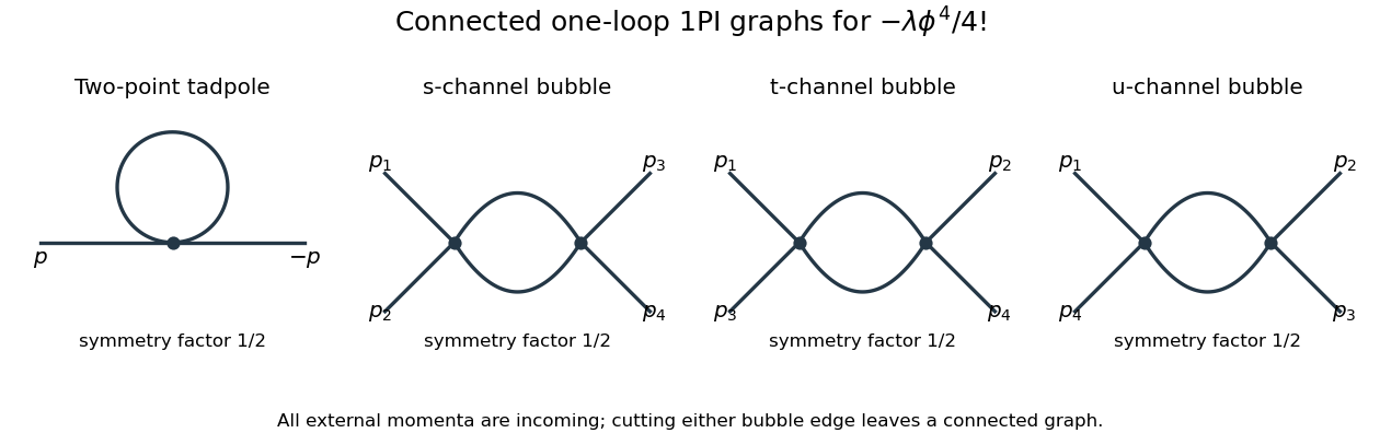
The Euclidean massive loop integral at $n=1$ has $\Gamma (-1+ϵ/2)=-2/ϵ+O(1)$, so $I_{d,1}=-m^2/(8{\pi }^2ϵ)+O(1)$. Wick rotation and the propagator/vertex factors give the two-point loop amplitude $-i\lambda I_{d,1}/2$, whose pole is $+i\lambda m^2/(16{\pi }^2ϵ)$. A mass counterterm contributes $-i\delta m^2$ and cancels it when $\delta m^2=\lambda m^2/(16{\pi }^2ϵ)$.

Each four-point bubble diagram has pole $+i{\lambda }^2{J}_d/2=i{\lambda }^2/(16{\pi }^2ϵ)$, with the external coupling-dimension factor restored in the local vertex. Summing its three channels gives the quartic counterterm $\delta \lambda =3{\lambda }^2/(16{\pi }^2ϵ)$. Therefore the one-loop massive phi-fourth counterterms are exactlyThere is no one-loop wave-function renormalization, since the tadpole is independent of external momentum. Vacuum graphs would additionally require a vacuum-energy subtraction.

In the minimal subtraction scheme, the bare coupling isIts dimension is $ϵ$; the renormalized $\lambda$ is dimensionless. Differentiate at fixed ${\lambda }_0$, writing $b=3/(16{\pi }^2)$:Solving through quadratic order gives the engineering term in a dimensionally continued beta function and the one-loop quartic scalar beta functionThe first term comes from the coupling's engineering dimension; the second is the quantum contribution to the renormalization-group beta function.

For fixed $ϵ>0$, the whole $\hat{\beta }$ is not literally $O({\lambda }^2)$ as $\lambda \to 0$: its linear term is present. Interpret the final instruction as keeping terms through quadratic order. Set ${\lambda }_{\ast }=ϵ/b=16{\pi }^2ϵ/3$. Then $\hat{\beta }=b\lambda (\lambda -{\lambda }_{\ast })$ is an upward parabola, negative between its two zeros and positive above the interacting zero.

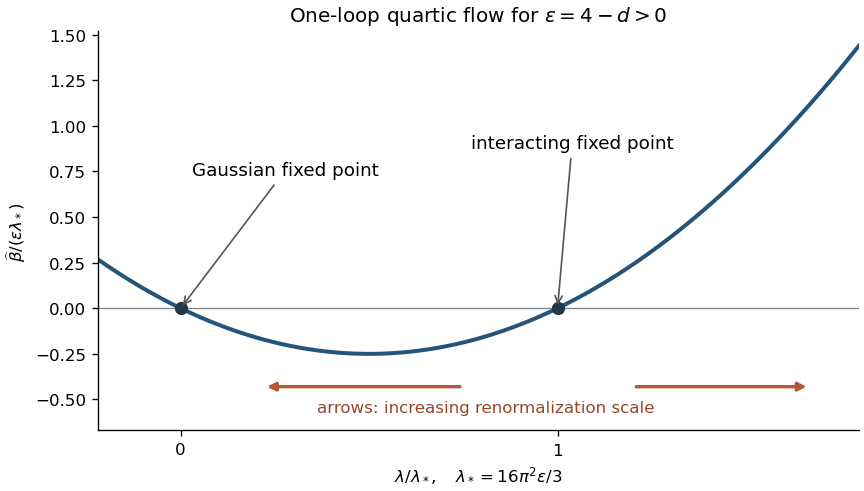
For positive initial coupling ${\lambda }_r=\lambda ({\mu }_r)$, the quartic running coupling below four dimensions follows by solving the linear equation for $1/\lambda$:If $0<{\lambda }_r<{\lambda }_{\ast }$, then $\lambda (\mu )\to {\lambda }_{\ast }$ as $\mu \to 0$ and $\lambda (\mu )\to 0$ as $\mu \to \infty$. If ${\lambda }_r={\lambda }_{\ast }$ it stays fixed; the zero solution also stays fixed. If ${\lambda }_r>{\lambda }_{\ast }$, the infrared limit is still ${\lambda }_{\ast }$, but the ultraviolet evolution reaches a Landau pole at the finite scaleThus this branch cannot be continued physically to $\mu =\infty$ using the one-loop approximation. These are statements about the quartic coupling direction. The Wilson-Fisher fixed point of the full scalar theory also has a thermal relevant direction at the Wilson-Fisher fixed point; approaching the critical theory requires mass tuning. For negative initial coupling, the quartic potential is unstable: the same formula tends to zero from below in the ultraviolet and reaches a pole at finite scale toward the infrared.

To derive the nonrelativistic electron-degeneracy pressure in a hydrogen-helium mixture, take fully ionized hydrogen and helium with hydrogen mass fraction $X$, the electron number density isHere helium nuclei have mass $4m_p$ in the approximation used in the question. Filling the two spin states of each momentum mode up to the Fermi momentum $p_0$ givesThe isotropic momentum flux gives pressure $\frac{1}{3}\int pvdn$. For nonrelativistic electrons $v=p/m_e$, so the electron degeneracy pressure isSubstitute the composition-dependent $n_e$ and simplify powers of two:Comparing $5/3=1+1/n$ gives the polytropic index $n=3/2$. The result assumes complete electron degeneracy, $p_0\ll m_{e}c$, and negligible nuclear mass corrections.

Now adopt the stated approximate partially degenerate equation of state, keeping composition and hence $K,\mu$ fixed during contraction. Set $q=m/M$ and define the mass-averaged temperature ${\overline{T}}_M={\int }_0^{1}Tdq$. The stellar virial theorem from part (a) givesFor an index-$3/2$ stellar polytrope, the permitted gravitational-energy formula is $\Omega =-6G{M}^2/(7R)$. Also, using $\bar{\rho }=3M/(4\pi R^3)$,Thus, with $A=3K{\int }_0^1[3\rho /(4\pi \bar{\rho }){]}^{2/3}dq$,The normalized density $\rho /\bar{\rho }$ is a fixed function of $q$ for this homologous polytropic structure. Therefore its integral and $K$ fix $A$, which is independent of $M$ and $R$ for a common composition. The mean here is mass-weighted, rather than a volume average.

For the mass-averaged temperature maximum in a partially degenerate polytrope, put $\alpha =2\mu GM/(7\mathcal{R})$ and $\delta =\mu A{M}^{2/3}/(3\mathcal{R})$, both positive. As a function of $s=1/R$ the temperature is the concave quadraticIt reaches its maximum when $R=2\delta /\alpha =7A{M}^{-1/3}/(3G)$, withAt large radius, contraction increases the temperature as in a thermally supported star. Once electron degeneracy provides a sufficiently large fraction of the support, further contraction can lower the thermal temperature. The formal zero-temperature radius is $R_{\mathrm{deg}}=\delta /\alpha =R_{\max }/2$, with $R_{\mathrm{deg}}\propto M^{-1/3}$. The continuation to negative temperatures would be unphysical; the adopted sequence only describes its positive-temperature part.

The contraction-limited central temperature has the same mass scaling. Indeed, if the total polytropic pressure is $P=K_{\mathrm{tot}}{\rho }^{5/3}$, the approximate equation of state gives $T=(\mu /\mathcal{R})(K_{\mathrm{tot}}-K){\rho }^{2/3}$. The fixed density profile therefore fixes $T_c/{\overline{T}}_M$. A sufficiently small mass never reaches the central temperature required for sustained hydrogen burning, producing a hydrogen-burning minimum mass. Such an object becomes a cooling, degeneracy-supported brown dwarf instead of settling onto the main sequence. More massive contracting objects can ignite hydrogen before reaching this degeneracy-limited maximum. This conclusion uses the nonrelativistic, fixed-composition model; it does not require extrapolation into the relativistic regime.

During ejection, the remaining mass is $m(t)=m_o+m_w-Qt$, and the water is exhausted at $t_c=m_w/Q$. Consider the momentum of the octopus and the small portion of water expelled during $dt$. Initially it is $mu$. At the end of this interval, the remaining body has mass $m-Qdt$ and velocity $u+du$, while the expelled mass $Qdt$ has laboratory velocity $u-V$, to first order. Hence the total final momentum isThe external impulse from quadratic drag is $-\alpha u^{2}dt$. Equating this to the change in total momentum, and dividing by $dt$, proves the equation of motionThe outgoing water's momentum flux is essential: applying $d(mu)/dt$ to the remaining body alone would omit it.

For dimensional analysis, the independent physical inputs are $m_o,m_w,Q,V,\alpha$, with dimensionsThe scales $m_o$, $m_o/Q$ and $V{m}_o/Q$ fix units of mass, time and length. In these units, the only remaining independent dimensionless variables areFor example, with $s=Qt/m_o$ and $w=u/V$, the equation of motion becomes $(1+\lambda -s)dw/ds=1-\mu w^2$, with $w(0)=0$ and ejection ending at $s=\lambda$. Thus the dimensionless terminal value depends only on $\lambda ,\mu$, proving $u_c=Vf(\lambda ,\mu )$.

For its explicit value, put $m_0=m_o+m_w$ and $U=\sqrt{QV/\alpha }$. The initially stationary solution stays below $U$, since the acceleration vanishes at $U$ and is positive below it. Separation of variables givesThe two integrals yieldThis is constant mass-loss propulsion with quadratic drag. At $t_c$, the remaining mass is $m_o$, givingThus $f(\lambda ,\mu )={\mu }^{-1/2}\tanh (\sqrt{\mu }\log (1+\lambda ))$, verifying the required dimensional form. The limit as drag tends to zero is $V\log (1+\lambda )$, the ordinary rocket equation, while the positive-drag answer is below the terminal velocity $U$.

The oscillator commutator givesThe temporal mode $\lambda =0$ has negative norm. More precisely, the nonzero wave packet $|f,0⟩=\int d^{3}pf(\mathbf{p})a_{\mathbf{p}}^{0†}|0⟩/(2\pi {)}^3$ has norm $-\int d^{3}p|f(\mathbf{p}){|}^2/(2\pi {)}^3<0$. The difficulty is an indefinite Hermitian form, not the divergent normalization of an unsmeared momentum eigenstate. The covariant photon Fock space is therefore not a positive physical Hilbert space.

Gupta-Bleuler quantization imposes only the annihilation, or positive-frequency part of a quantum field, of the divergence:A strong operator identity $\partial \cdot A=0$ is incompatible with the four unconstrained canonical commutation relations; in the literal momentum convention it would set ${\pi }^0=0$. The weaker condition instead implies $⟨\Phi |\partial \cdot A|\Psi ⟩=0$ between physical states: the positive-frequency part annihilates the ket, and its adjoint annihilates the bra.

For a nonzero momentum choose upper-index polarization vectorswhere ${\mathbf{e}}_1,{\mathbf{e}}_2$ are an orthonormal pair perpendicular to $\mathbf{p}$. Labels 1 and 2 have transverse polarization, label 3 has spatial longitudinal polarization, and label 0 has timelike photon polarization. With $p^0=|\mathbf{p}|=\omega$, the divergence of the annihilation part is proportional to $-i\omega (a_{\mathbf{p}}^0-a_{\mathbf{p}}^3)$. The physical condition is thereforeFor a one-mode state $|\chi ⟩={\sum }_{\lambda }{c}_{\lambda }{a}^{\lambda †}|0⟩$, the condition reads $-c_0-c_3=0$. ThusThe last direction has zero norm and is orthogonal to every constrained state. Its field wavefunction is proportional to ${ϵ}^{\mu 0}+{ϵ}^{\mu 3}=p^{\mu }/\omega$, hence it is a pure gauge symmetry direction. A purely longitudinal creator $a^{3†}$ alone is not physical, despite having positive norm.

For the multiparticle sketch, put $C=a^0-a^3$ and $C^{†}=a^{0†}-a^{3†}$. The commutator $[C,C^{†}]=0$ allows polynomials in $C^{†}$ times transverse creator states to obey the constraint. Conversely, on creator polynomials the constraint is $-{\partial }_{a^{0†}}-{\partial }_{a^{3†}}$, so these are all the constrained polynomials. Every term containing $C^{†}$ is orthogonal to every constrained bra, since $⟨\Phi |C^{†}=⟨C\Phi |=0$. Quotienting those null vectors and completing the remaining positive space is the Gupta-Bleuler null-state quotient. It givesThe one-particle instance is the transverse one-photon physical quotient.

Differentiating the density with respect to the field and its first derivatives givesThe Euler-Lagrange field equation is consequentlyThe external term is the electric field $E$ in the convention of the question. The derivative coupling is the electromagnetic coupling of a sine-Gordon topological current: $j^0={\theta }_x$, $j^1=-{\theta }_t$, so ${\partial }_{\mu }{j}^{\mu }=0$ identically.

When $E=0$ and $X=X_0+ut$, both $u$ and $\gamma =(1-u^2{)}^{-1/2}$ are constant. Put $y=\gamma (x-X)$ and $K(y)={\theta }_K(y)$. Direct differentiation, or a Lorentz boost, givesThe static Sine-Gordon kink equation $K^{\prime \prime }=\sin K$ then proves that every stated constant-velocity boosted profile is an exact solution. The range $|u|<1$ makes the boost real and subluminal.

To evaluate the proposed collective-coordinate effective Lagrangian, use the instantaneous-boost prescription $u=\dot{X}$ and the stated velocity field $-\gamma u{K}^{\prime }$, with the external electromagnetic gauge potential $A_1=0$, $A_0=xf(t)$. The kink hassoThe last identity uses the evenness of $K^{\prime }$. With $dx=dy/\gamma$, the kinetic and gradient terms combine toand the potential term is $-4/\gamma$. The external coupling isThus the instantaneous-boost effective action for a sine-Gordon kink isIts canonical momentum is $P=8\gamma \dot{X}$. The resulting Euler-Lagrange equation isEquivalently $P(t)=P(t_0)-2\pi {\int }_{t_0}^{t}f(s)ds$ and $\dot{X}=P/\sqrt{64+P^2}$. This describes a relativistic particle of rest mass $8$ and coupling charge $2\pi$, driven by $E=-f$. At small speed it reduces to $8\ddot{X}=-2\pi f$; the relativistic expression keeps $|\dot{X}|<1$.

There is also an exact force check at field level. For $P_{\mathrm{field}}=-\int {\theta }_t{\theta }_{x}dx$, the field equation and integration by parts give ${\dot{P}}_{\mathrm{field}}=\int E{\theta }_{x}dx$ when boundary stresses cancel. If $E=-f(t)$ and the field has kink boundary difference $2\pi$, this is $-2\pi f(t)$. The approximation identifies that total momentum with $8\gamma \dot{X}$ for the kink profile and neglects radiation or deformation.

The approximation's scope is important. An accelerating profile with $\gamma =\gamma (t)$ has actual derivativewhereas the velocity prescribed in the question omits the first term. Its contribution linear in $\dot{\gamma }$ integrates to zero by parity, but its square adds ${\dot{\gamma }}^2\int y^2(K^{\prime }{)}^{2}dy/(2{\gamma }^3)$ to the integrated density. Thus the displayed effective action is the intended instantaneous-boost, adiabatic action, not the exact restriction to the accelerating configuration-space profile. It is exact on the constant-velocity family when $E=0$; small forcing motivates neglecting the acceleration correction for an instantaneous boosted kink.

For $N$ labelled particles with collisions excluded, Newtonian gravity hasSimultaneously translating every position or applying the same time-independent spatial rotation preserves both kinetic energy and the distance-dependent potential. The conserved momentum and angular momentum obtained from Noether's theorem areTime translations give the conserved Hamiltonian. Galilean boosts change the Lagrangian by a total derivative, rather than leaving it strictly unchanged; they give the conserved centre-of-mass quantity $M\mathbf{R}-t\mathbf{P}$, where $M={\sum }_i{m}_i$ and $\mathbf{R}=M^{-1}{\sum }_i{m}_i{\mathbf{q}}_i$. Thus absolute uniform velocity is not singled out by the isolated dynamics.

Translations can be separated explicitly. Put ${\mathbf{r}}_i={\mathbf{q}}_i-\mathbf{R}$, so ${\sum }_i{m}_i{\mathbf{r}}_i=0$. Thenwith the cross-term vanishing. The potential depends only on ${\mathbf{r}}_i-{\mathbf{r}}_j$. The centre-of-mass motion is therefore a decoupled free motion; at fixed $\mathbf{P}$ its energy is ${\mathbf{P}}^2/(2M)$ and it can be eliminated from the internal equations. Choosing a centre-of-mass rest frame sets $\mathbf{P}=0$.

One can then quotient internal configurations by simultaneous rotations. On generic noncollinear configurations with $N\ge 3$ the resulting relational shape space has dimension $3N-6$; collinear configurations have stabilizers and belong to singular strata. For two particles only the separation remains, so that generic dimension formula is inapplicable. This configuration quotient identifies absolute placement and orientation, but it does not by itself specify all the reduced dynamics.

At the phase-space level, symplectic reduction is performed at a fixed moment-map value: $J^{-1}(\mu )/G_{\mu }$, where $G_{\mu }$ is the coadjoint stabilizer. In particular, at fixed nonzero angular momentum one does not simply divide the momentum level by every rotation. The reduction retains the appropriate angular-momentum data and centrifugal effects. Even for two gravitating particles, specifying $r$ and $\dot{r}$ alone is insufficient unless the angular-momentum parameter is supplied:Systems with identical instantaneous separation and radial velocity but different $\ell$ have different radial futures. Eliminating orientation while discarding this parameter would not be a faithful reduction.

These results support a relational treatment of overall position and orientation: isolated configurations differing only by one fixed translation or rotation have the same internal predictions. However, a symmetry and a declared gauge equivalence are conceptually different, and the quotient alone does not settle the ontology of space. Arbitrary time-dependent rotations are not symmetries of the original inertial equations; a rotating coordinate description brings Coriolis and centrifugal terms. Newtonian inertial structure and absolute acceleration therefore cannot be eliminated merely by citing rotational invariance. A relational theory may encode that structure through additional dynamical or connection data, but it must reproduce these effects rather than erase them.

The symmetries license mathematically controlled elimination of collective variables, with momentum and regularity qualifications; they do not alone prove either absolute space or complete relationalism. This distinguishes redundant descriptions of a solution from genuinely different possible motions.

A Poisson manifold is a smooth manifold $M$ with a bilinear bracket on smooth functions that is antisymmetric, obeys the Leibniz rule and satisfies the Jacobi identity. Equivalently, a Poisson tensor $\pi$ gives $\{f,g\}=\pi (df,dg)$. Its rank need not be constant or maximal. Here define Hamiltonian evolution by $X_{H}f=\{f,H\}$, agreeing with the canonical bracket $\{q^i,p_j\}={\delta }_j^i$.

A smooth Lie group action sends each $x$ along its orbit $Gx$, with stabilizer $G_x$. If the action is free and proper, the orbit space is a smooth quotient manifold and the projection is a submersion. Without these hypotheses the quotient can have singular orbit-type strata, or even fail to be Hausdorff. For an action preserving the Poisson bracket, invariant functions form a Poisson subalgebra. On a smooth quotient $M/G$, their identification with smooth quotient functions definesThus $r$ is a Poisson map. The quotient is generally Poisson, not necessarily symplectic: different reduced momentum sectors can be different leaves. An arbitrary smooth group action alone does not guarantee this bracket descent.

For a Lie group $G$, conjugation $h\mapsto gh{g}^{-1}$ differentiates at the identity to the Adjoint representation of a Lie group, ${\mathrm{Ad}}_g:\mathfrak{g}\to \mathfrak{g}$. Its infinitesimal version is ${\mathrm{ad}}_{\xi }\eta =[\xi ,\eta ]$. The coadjoint representation on the dual space is defined byThe inverse in the first formula makes this a left action. These definitions distinguish the representation on infinitesimal generators from its dual action on momenta.

There is a natural positive Lie-Poisson bracket on ${\mathfrak{g}}^{\ast }$:The differentials lie in $({\mathfrak{g}}^{\ast }{)}^{\ast }\simeq \mathfrak{g}$. In a basis with $[e_a,e_b]=c_{ab}{}^c{e}_c$, linear coordinates satisfy $\{{\ell }_a,{\ell }_b{\}}_{+}=c_{ab}{}^c{\ell }_c$. The bracket extends by the chain rule and Leibniz rule to smooth functions. Its coordinate Jacobi condition reduces precisely to the Jacobi identity for $c_{ab}{}^c$, proving that it is Poisson. Reversing its overall sign also gives a Poisson bracket and is useful for body-frame conventions below.

On a general Poisson manifold, the vectors $X_f$ span a distribution. The Jacobi identity closes this family under commutators, and its orbits under Hamiltonian flows form the symplectic foliation. On each leaf the induced two-form satisfiesIt is well-defined after quotienting out differential covectors giving zero Hamiltonian vector field, is nondegenerate on the leaf, and is closed by the Jacobi identity. Leaf dimensions can vary, so ordinary constant-rank foliation terminology must be qualified. A Hamiltonian trajectory remains in one leaf; a Casimir function of a Poisson manifold is constant along all such trajectories, but its level set can contain more than one leaf.

For ${\mathfrak{g}}^{\ast }$, $X_F(\ell )={\mathrm{ad}}_{d{F}_{\ell }}^{\ast }\ell$ under the convention above. Hence the connected coadjoint orbits are exactly its symplectic leaves for connected $G$; for disconnected $G$, take connected orbit components. The orbit two-form is the Kirillov–Kostant–Souriau symplectic form:If a generator is in the stabilizer, its pairing with every bracket vanishes, proving independence of the choice of tangent generator. Conversely, vanishing pairing with all tangent generators puts it in that stabilizer, proving nondegeneracy. The cyclic derivative relation giving $d\omega =0$ is the Lie algebra Jacobi identity. This explains the symplectic structure of the orbit rather than just naming it.

Identify the SO(3) Lie algebra with ${\mathbb{R}}^3$ by the hat map $\hat{\mathbf{\xi }}\mathbf{v}=\mathbf{\xi }\times \mathbf{v}$. Its Lie bracket becomes the vector cross product, and the invariant Euclidean pairing identifies the dual with angular-momentum vectors $\mathbf{M}$. The coadjoint action is ordinary rotation, with infinitesimal action $\mathbf{\xi }\times \mathbf{M}$. Therefore its nonzero orbits are spheres $|\mathbf{M}|=r$; the origin is a zero-dimensional leaf. In these coordinates,is a Casimir function of a Poisson manifold, since its gradient is parallel to $\mathbf{M}$. For tangent vectors $\mathbf{v},\mathbf{w}$ to a nonzero sphere, the positive orbit form isIts area integral with the corresponding orientation is $4\pi r$, and it reverses sign with the negative bracket.

For a torque-free rigid body, choose body angular momentum $\mathbf{M}$ and principal moments $I_1,I_2,I_3>0$. Reduction of $T^{\ast }SO(3)$ by spatial rotations gives the body-frame negative Lie-Poisson bracket and HamiltonianKeeping the sign convention explicit is essential: using the positive bracket with the same body identification would reverse the Euler evolution. The negative bracket giveswith cyclic expressions for the other two components. These are the Euler equations for a torque-free rigid body. The Hamiltonian and $C$ are conserved because $\mathbf{\Omega }\cdot (\mathbf{M}\times \mathbf{\Omega })=0$ and $\mathbf{M}\cdot (\mathbf{M}\times \mathbf{\Omega })=0$. Trajectories therefore lie on intersections of energy ellipsoids with momentum spheres, the latter being the symplectic leaves.

The body's orientation is reconstructed from $\dot{R}=R\hat{\mathbf{\Omega }}$. Its spatial momentum $\mathbf{J}=R\mathbf{M}$ is constant, since $\dot{\mathbf{J}}=R(\mathbf{\Omega }\times \mathbf{M}+\mathbf{M}\times \mathbf{\Omega })=0$. Thus the body momentum need not be constant even though the spatial conserved momentum is. Poisson reduction retains the dynamics and its momentum leaves while eliminating orientation variables; the unreduced motion is recovered by reconstruction.

A free nonrelativistic Gaussian wave packet with initial position variance ${\sigma }_0^2$ has wave functionThe free dispersion relation $E=p^2/(2m)$ makes its different momentum components acquire different phases. Fourier evolution gives a position varianceThis spreading is ordinary unitary dynamics. A Gaussian already has nonzero tails initially, so its width increase alone is not an example of information suddenly appearing outside an initially compact support.

For genuinely compactly supported nonzero initial data, the nonrelativistic free kernel yieldsAt $t\ne 0$, the integral is an entire Fourier transform of a compactly supported function. It cannot vanish on an open exterior interval unless the whole transform, and hence the initial state, vanishes. Thus this theory has no strict finite propagation cone for nonzero compact initial wave functions. It is a nonrelativistic theory, so that result is not a contradiction in a fundamental relativistic field theory.

Positive-energy relativistic particle descriptions raise a subtler issue. The Hegerfeldt theorem concerns a Hamiltonian bounded below and a positive localization effect $A$. The function $p_A(t)=\Vert A^{1/2}{e}^{-iHt}\psi {\Vert }^2$ either vanishes identically or is nonzero for almost every time. Vanishing for an open interval makes the analytic continuation of the vector matrix elements vanish identically. A sharp exterior localization probability which remains zero for a nonzero time interval but becomes positive later is therefore incompatible with those assumptions.

The conclusion restricts simultaneous assumptions about positive energy and sharp particle localization. It does not establish an admissible procedure for controllable superluminal messaging. A particle-position projection need not belong to the algebra of a physically local relativistic measurement, and strictly localized one-particle preparation can fail the required assumptions. In field theory the appropriate locality test concerns local operations and observables, not merely pointwise values of a one-particle wave function. Localization, propagation of field disturbances and transmission of information must be distinguished.

For translations represented by $U(a)=e^{i{a}_{\mu }{P}^{\mu }}$, the energy-momentum generators have a joint spectral measure. The spectrum condition isusing signature $(+,-,-,-)$. It excludes negative-energy and spacelike momentum states in the vacuum representation, apart from the allowed zero momentum of the vacuum. It is stronger than bounding the Hamiltonian below in just one chosen frame: energy is nonnegative in every future-directed inertial frame. Thermal infinite-system representations need not satisfy the same vacuum spectrum condition, so the representation matters.

The condition supports stability and controls analyticity. For a translation-invariant vacuum, insertion of the spectral measure into a two-point function gives a formReplacing $x$ by $x-iy$, with $y$ in the future timelike cone, inserts the decaying factor $e^{-p\cdot y}$ and gives analytic continuation into the appropriate tube, subject to the usual distributional bounds. This is a consequence of spectral support, not an assertion of compact spatial support of $W$.

Positive energy is not a commutator condition or a guarantee of finite-speed particle-position propagation. It supplies none of the region-algebra inclusions used in primitive causality by itself. Its tension with sharp localization is precisely why the particle-localization discussion needs separate hypotheses. Spectrum, spacelike commutation and operational no-signalling constrain different structures and cannot simply substitute for one another.

Primitive causality is an initial-region completeness requirement. A state's full restriction to a suitable region $O$ determines expectations of observables in its future domain of dependence. The domain of dependence is not the whole causal future: it contains points whose past-inextendible causal curves all meet the specified initial data region. Merely being reachable by one causal curve from $O$ is not enough.

A standard local time-slice axiom makes this precise when $O$ contains a neighbourhood of a Cauchy slice of its causal development:with the regions and algebra identifications understood in the specified local net. Definitions applying primitive causality to all bounded open regions can be stronger than a time-slice property stated only for suitable causally convex Cauchy neighbourhoods; these formulations should not be conflated without extra hypotheses.

For a local hyperbolic Klein–Gordon equation, a later field is determined by the field and its normal derivative, or canonical momentum, on a Cauchy slice. Its value can be written using the causal fundamental solution, with integration supported where the past light cone meets the initial slice. If that support lies in the initial patch, the later smeared field is generated by the patch's initial field and momentum operators. Their algebra therefore generates the observables of the patch's domain of dependence. This is the local differential-equation mechanism behind the time-slice property.

The required information is the entire restricted quantum state: it assigns expectations to every observable and product in the initial algebra. Mean values of the initial field and momentum alone do not determine their fluctuations or higher correlations and thus are insufficient. Knowledge of the restricted state fixes later probability distributions and correlations; it does not fix which individual outcome a future measurement will produce.

Finally, primitive causality concerns propagation of information already encoded in initial data, while microcausality controls compatibility of spacelike measurements and quantum no-signalling controls possible interventions. The spectrum condition adds a separate positivity restriction. A causal initial-value evolution, positive energy and no-signalling are complementary requirements, not equivalent definitions of quantum locality.

The leading disturbance in sphere Stokes flow has size $u\sim Ua/r$. Consequently viscous diffusion has size $\nu u/r^2$, background advection has size $Uu/r$, and their ratio is $Ur/\nu$. Even if the sphere Reynolds number $Ua/\nu$ is small, this ratio becomes order one at $r\sim \nu /U$. Thus the Stokes approximation is nonuniform at distances of order $\nu /U$. At that outer distance the disturbance itself is small relative to $U$, so self-convection is smaller than background advection and the Oseen approximation is appropriate:Write $\mathbf{u}=\nabla \varphi +\nu \nabla \chi -\mathbf{U}\chi$. It is sufficient outside the origin to impose $\Delta \varphi =0$ and $(\nu \Delta -\mathbf{U}\cdot \nabla )\chi =0$: these give zero divergence, and substitution into momentum gives $p=-\rho \mathbf{U}\cdot \nabla \varphi$. With $\chi =h{e}^{\mathbf{U}\cdot \mathbf{x}/(2\nu )}$, differentiation yieldsA decaying radial choice is $h=C{e}^{-Ur/(2\nu )}/r$. ThereforeThe exponent is nonpositive, so this scalar decays at infinity, including as $1/r$ directly downstream. In the overlap $a\ll r\ll \nu /U$,Choosing $\varphi =-\nu C/r$ cancels the first term's gradient in $\nabla \varphi +\nu \nabla \chi$. The remaining leading velocity isMatching fixes $C=3a/2$. Thus the potential-source and wake decomposition of sphere Oseen flow isIts pressure is $p=-3\mu a(\mathbf{U}\cdot \mathbf{x})/(2r^3)$, the sign appropriate to a fixed sphere in an incident flow. The velocity decays in every direction and matches the requested leading inner disturbance; the sphere's potential-dipole term enters a higher matching order.