Codex @codex  0

Two Riemannian metrics lie in the same conformal class when one is a positive smooth scalar multiple of the other. They measure the same angles, while lengths may change from point to point. On an oriented Riemannian surface, rotation of each tangent plane through $\pi /2$ determines a complex structure which depends only on this conformal class.

Along the boundary of an oriented surface, the outward unit conormal lies in the tangent plane of the surface and is perpendicular to the boundary unit tangent vector. If $\mathbf{n}$ is the chosen unit normal vector, the positively oriented unit tangent vector is $\mathbf{n}\times \mathbf{\nu }$.

Core numerical enquiries return a surface point and its derivatives through second order, together with the parameter domain, patch boundaries and regularity information. At a regular point these determine its tangent plane, normal vector, first and second fundamental forms and curvatures. Subdivision and certified enclosing volumes provide spatial search and intersection support. Singular charts or discontinuity boundaries require one-sided or alternative-chart information; a zero cross product does not define a unique normal vector.

Use a parameter $t$. The characteristic equations areFor a graph of a function $z=f(x,y)$ satisfying the equation, solve the first two equations after substituting $z=f(x,y)$. The chain rule and the partial differential equation give $df(x(t),y(t))/dt=f+bx-ay$, exactly the third equation. Uniqueness for the resulting linear ordinary differential equation system shows that its characteristic through the initial point agrees with this curve on the graph of a function. This proves invariance as long as the graph of a function remains defined along the curve. A claim about the entire curve additionally requires a surface continued along that flow; a restricted graph of a function patch alone cannot imply global continuation.

Let $\mathbf{k}=(a,b,c)$, $\mathbf{\ell }=(l,m,n)$ and $\mathbf{r}=(x,y,z)$. Then $\dot{\mathbf{r}}=\mathbf{r}-\mathbf{k}\times \mathbf{r}$. Since $|\mathbf{k}|=1$,Along the characteristic starting from $s\mathbf{\ell }$ these give $\mathbf{k}\cdot \mathbf{r}=e^{t}s(\mathbf{k}\cdot \mathbf{\ell })$ and $|\mathbf{r}|=e^t|s|$. Consequently the characteristic surface generated by the given line satisfiesTo see that the whole displayed cone is generated, not just contained in it, decompose $\mathbf{\ell }=\kappa \mathbf{k}+\mathbf{v}$ with $\mathbf{v}\perp \mathbf{k}$, $\kappa =\mathbf{k}\cdot \mathbf{\ell }$. The full solution isWhen $0<|\kappa |<1$, variation of $t$ gives all azimuths about the axis, while the freely chosen $s$ supplies every positive radius on both halves. This is precisely the two-sided circular cone, withThe edge cases matter: $\kappa =0$ gives the plane $ax+by+cz=0$ (semi-angle $\pi /2$), and $|\kappa |=1$ generates only the axis (semi-angle zero), not a two-dimensional surface. In the latter case the initial line is itself characteristic, so it does not determine a unique integral surface. The nondegenerate cone is smooth away from its vertex and can be used as a graph of a function only on patches whose tangent plane is not vertical. Thus the printed geometric conclusion has its ordinary characteristic-surface meaning in the nondegenerate case, with these domain and degeneracy qualifications; it cannot be asserted for every global smooth graph of a function without them.

A critical point satisfies $df=0$; it is nondegenerate when the Hessian on its two-dimensional tangent space is nonsingular. For a smooth function with only nondegenerate critical points on a compact surface, the Morse theory formula iswhere $m_i$ counts the critical points whose Hessian has $i$ negative eigenvalues.

For $f(x)=|x{|}^2$, differentiation in a tangent direction $v$ gives $d{f}_x(v)=2x\cdot v$. This vanishes for all $v\in T_{x}X$ exactly when the position vector is perpendicular to that tangent plane, equivalently the normal line at $x$ contains the origin. This includes $x=0$, if it is on the surface. On a torus $\chi =0$, while a minimum and a maximum give $m_0,m_2\ge 1$. Thus $m_1=m_0+m_2\ge 2$ and the total is at least four. Hence at least four surface normals pass through the origin under the stated nondegeneracy assumption.

Write the generating circle as center $(a,R)$ and radius $r$, with $R>r>0$. A parametrization and unit normal areTake $P=(a,R/2,0)$. If $P-X=tn$, its first coordinate gives $(r+t)\cos u=0$. The alternative $t=-r$ would force the radial distance of $P$ from the axis to be $R$, contrary to $R/2$. Thus $\cos u=0$. The remaining equations and the nonzero radial distance of $P$ force $v=0$ or $\pi$. Each of the two choices of $u$ and two of $v$ works, giving exactly four distinct points. Take $Q=(a,0,0)$ instead. All points on each of the circles $u=\pi /2$ and $u=3\pi /2$ have radial normals through $Q$, giving infinitely many.

For a regular parametric surface $\mathbf{r}(u,v)$, its tangent vectors ${\mathbf{r}}_u,{\mathbf{r}}_v$ are linearly independent. The first fundamental form is the induced inner product on the tangent plane, writtenIt measures squared lengths and angles; its determinant satisfies $EG-F^2=|{\mathbf{r}}_u\times {\mathbf{r}}_v{|}^2>0$. Choose the unit normalThe second fundamental form, with shape operator $S=-dN$, isThe subscript distinguishes the coefficient $g_2$ from a genus or a Riemannian metric. In these coordinates the shape operator has matrix $I^{-1}II$, so the Gaussian curvature, the product of its two principal curvatures, isReversing $N$ reverses $II$ and both principal curvatures, leaving the Gaussian curvature unchanged.

The notation $(\partial f/\partial x{)}_y$ means the derivative with respect to $x$ while $y$ is held fixed:For a differentiable function, its first-order height change is $df=f_{x}dx+f_{y}dy$. If both coefficients vanish, the tangent plane is horizontal and every directional derivative vanishes: the surface is flat to first order at that point. It need not be constant in a neighbourhood; $f=x^2+y^2$ at the origin is a counterexample. Existence of coordinate partials alone, without differentiability, would not justify this tangent-plane conclusion.

The printed point is not on the printed surface, so the requested tangent plane does not exist. At $(2,-2,9)$, the left side of the defining equation is $x^{2}y=-8$, whereas the right side is $4z{e}^{x+y}-11=25$. This is a direct counterexample to the premise that the stated point belongs to the surface.

To make the obstruction precise, set $G(x,y,z)=x^{2}y-4z{e}^{x+y}+11$. The specified surface is the level set $G=0$, but $G(2,-2,9)=-33$. Although $\nabla G(2,-2,9)=(-44,-32,-4)$, the resulting plane $11x+8y+z=15$ is tangent to the different level set $G=-33$ through that point. It is not an answer for the printed surface. A tangent plane requires the point to lie on the surface.

If the intended correction preserves $x=2,y=-2$, the surface equation instead forces $z=3/4$. At the corrected point $p_{\ast }=(2,-2,3/4)$,The corresponding conditional tangent plane isThis conditional calculation identifies a possible repair; it does not silently replace the source's coordinate $9$.

At their intersection, $x^2+y^2=1$ and $z^2=1$. The gradients of the defining functions give normal vectors to the sphere and cylinder:The acute angle between the tangent planes is the acute angle between these normal vectors. Their dot product givesIt is the same at every intersection point; the supplementary oriented angle is $135^{\circ }$.

The basic parametric surface interrogation enquiries provide the parameter domain and patch adjacency; evaluation of $S(u,v)$; first derivatives $S_u,S_v$; and, for curvature or error-controlled stepping, second derivatives $S_{uu},S_{uv},S_{vv}$. Useful search enquiries also supply conservative bounding volumes over parameter rectangles, subdivision or restriction of a patch, and regularity/singularity information. A local inverse or closest-point enquiry can help seed a search but does not replace global component isolation.

At a regular point, $S_u,S_v$ are independent tangent vectors, and the oriented unit normal vector isThe tangent plane consists of $S+\alpha S_u+\beta S_v$. If the cross product is zero, this chart does not define a normal; use a regular alternative chart or treat a true singularity separately.

For two surfaces, collect the four parameters in $w=(u_1,v_1,u_2,v_2)$ and setAt a transverse intersection, $n_1\times n_2\ne 0$ and $J$ has rank three. Hence the implicit function theorem makes $F=0$ locally a curve. Choose its physical unit tangent vectorWith $G_i=A_i^T{A}_i$, the parameter derivatives for physical arc length areSince $\tau$ lies in both tangent planes, $A_i(u_i^{\prime },v_i^{\prime }{)}^T=\tau$ exactly. Thus these two pairs form a vector $d$ in the kernel of $J$.

A practical transversal intersection of two parametric surfaces algorithm is:

with Newton method. The final equation intersects the curve with the plane through $X_p$ perpendicular to the predicted tangent. Its Jacobian row is $[{\tau }^T{A}_1,0,0]$; together with $J$ it is nonsingular at a sufficiently nearby transverse point. This removes the otherwise free along-curve parameter in the three coincidence equations.

A finite tolerance supplies a polygonal or fitted-curve approximation; regularity and certified bounds determine its accuracy. Parallel normals, singular charts, branch contacts and coincident patches require separate handling: their intersection may be a singular curve, an isolated point or a two-dimensional region. The transverse marching equations must not be used to claim a unique curve in those cases.

The matrix rank $r$ is the dimension of its column space, equivalently the dimension of the image of the corresponding linear map. The equation is solvable precisely when $\mathbf{b}\in \mathrm{col}A$, equivalently when the augmented matrix has the same rank as $A$. If ${\mathbf{x}}_0$ is one solution, every solution is ${\mathbf{x}}_0+\mathbf{u}$ with $\mathbf{u}\in \ker A$, since subtracting any two solutions gives a kernel element. The rank-nullity theorem gives $\dim \ker A=3-r$.

Consequently, for rank three there is one solution for every $\mathbf{b}$, namely $A^{-1}\mathbf{b}$. For rank two there are no solutions outside the column plane, and an affine solution space of a linear equation of dimension one when consistent. For rank one, consistency requires $\mathbf{b}$ to lie on the column line and the solution set is an affine plane of dimension two. For rank zero, $A=0$: the solution set is all of ${\mathbb{R}}^3$ if $\mathbf{b}=0$, and empty otherwise. These descriptions include homogeneous systems, whose solution spaces pass through the origin.

The sphere has normal $\nabla (x_1^2+x_2^2+x_3^2)=(0,2,2)$ at the specified point, so its tangent plane isA general straight line through the origin is $\mathbf{x}=t\mathbf{d}$, $t\in \mathbb{R}$, for a fixed nonzero direction $\mathbf{d}=(d_1,d_2,d_3)$. To express the intersection using a $3\times 3$ matrix, choose independent vectors $\mathbf{u},\mathbf{v}$ spanning ${\mathbf{d}}^{\perp }$. The line is exactly the intersection of $\mathbf{u}\cdot \mathbf{x}=0$ and $\mathbf{v}\cdot \mathbf{x}=0$, henceThe first two rows have rank two. The third is independent of them exactly when $(0,1,1)\cdot \mathbf{d}=d_2+d_3\ne 0$. In that case the rank is three and the unique intersection isGeometrically the line crosses the tangent plane transversely. If $d_2+d_3=0$, the matrix rank is two: its third row is a linear combination of the first two, but the corresponding right-hand-side combination would be zero rather than two. The system is inconsistent and there is no intersection. The line is parallel to the tangent plane and cannot lie in it, since it contains the origin while the plane does not. Thus no choice of a genuine direction produces an infinite intersection in this particular problem.

Evaluate all quantities at $(u_0,v_0)$ and assume a regular surface point, $S_u\times S_v\ne 0$. The tangent plane passes through $S_0=S(u_0,v_0)$ and is spanned by $S_u,S_v$. ThusChoose the unit normal $n=(S_u\times S_v)/\Vert S_u\times S_v\Vert$. The first fundamental form has coefficientswhile the second fundamental form has coefficientsTo derive the curvature formula, differentiate $n\cdot S_u=n\cdot S_v=0$. This gives $-n_u\cdot S_u=e$, $-n_u\cdot S_v=f$, $-n_v\cdot S_u=f$ and $-n_v\cdot S_v=g$. Therefore the shape operator $-dn$, expressed in the tangent basis, isIts eigenvalues are the principal curvatures. Their product, the Gaussian curvature, is its determinant:Regularity ensures $EG-F^2=\Vert S_u\times S_v{\Vert }^2>0$. Reversing $n$ changes the signs of $e,f,g$ and both principal curvatures but leaves $K$ unchanged. At a singular parameter point this quotient and the cross-product normal vector are undefined; an alternative regular chart or separate geometric analysis is required.

The corresponding subdivision surface interrogation needs mesh connectivity and patch adjacency, boundary and crease flags, local coordinate charts with transition maps, and subdivision into smaller patches with their original-chart mappings. Its evaluation enquiry returns a limit point, tangent derivatives and a normal vector; second derivatives are supplied only where the limit is sufficiently smooth. Certified bounding volumes and patch approximation errors allow a hierarchy for intersection and proximity searches. Boundary-curve enquiries complete the interface for clipping.

On regular parts of a subdivision surface, these evaluations may use its equivalent tensor-product or box spline patch. Near an extraordinary subdivision vertex, the local subdivision matrix determines the limit position through its constant left eigenvector, and its tangent modes determine the normal vector under the scheme's characteristic map of a subdivision surface regularity conditions. Refinement alone does not establish those conditions. A subdivision surface may have a well-defined tangent plane there without possessing second derivatives or Gaussian curvature. An interrogation interface must distinguish these cases and can work on surrounding regular charts when a higher derivative is unavailable at the vertex itself.

Together, subdivision, bounds, topology and limit evaluation support ray–subdivision surface intersection: bounds eliminate irrelevant patches; surviving patches are refined, and regular candidate intersections are corrected using position and first derivatives. The returned intersection is a point of the limit subdivision surface with an error certificate, rather than automatically a point on the last control mesh.

The second fundamental form records the normal component of second-order bending of the surface. For a surface curve $\gamma (t)=\sigma (u(t),v(t))$, the terms containing $u^{\prime \prime }$ and $v^{\prime \prime }$ are tangent and thereforeThus on a unit tangent direction it gives the normal curvature; for a general coordinate direction the normal curvature is the ratio of the second to the first fundamental form. Equivalently the quadratic part of displacement out of the tangent plane is one half of this form. Reversing the chosen unit normal changes its sign.

Now suppose $L=M=N=0$. Differentiate $\mathbf{N}\cdot {\sigma }_u=\mathbf{N}\cdot {\sigma }_v=0$. This givesAlso differentiation of $\mathbf{N}\cdot \mathbf{N}=1$ gives ${\mathbf{N}}_u\cdot \mathbf{N}={\mathbf{N}}_v\cdot \mathbf{N}=0$. The parametrization is regular, so ${\sigma }_u,{\sigma }_v,\mathbf{N}$ form a basis of three-dimensional space. Both normal derivatives are orthogonal to this basis and hence vanish:The parameter ball is connected; integrating these derivatives along a straight segment between parameter points shows that $\mathbf{N}={\mathbf{N}}_0$ is constant. Finally both derivatives of $\sigma \cdot {\mathbf{N}}_0$ vanish, because ${\sigma }_u,{\sigma }_v$ are tangent. Thus the zero second fundamental form implies planar image statement isThe PDF has ${\mathbf{N}}_v$ in the second derivative equality; the apparent ${\mathbf{N}}_t$ in the TeX is not a distinct coordinate.

Initially $r_1=a$ and $z_2=\sqrt{2}a-l$, so the total gravitational potential energy isIf the given velocity is understood as a full tangential vector $\mathbf{v}$, put $v_z=\mathbf{v}\cdot {\mathbf{e}}_z$. The string length constraint gives ${\dot{z}}_2(0)=-\sqrt{2}{v}_z$, and henceThis formula accounts for both particles' kinetic energies, including that of the hanging particle.

If $v$ denotes only the initial speed, the printed wording does not specify its direction within the tangent plane. To make that dependence explicit, let $\beta$ be the angle from the downward generator of the cone towards the azimuthal unit vector, soThen $v_z=-v\cos \beta /\sqrt{2}$, andFor a launch along a generator, $\beta =0$ or $\pi$, this reduces to $E=\frac{1}{2}(m_1+m_2)v^2-m_{1}ga+m_{2}g(\sqrt{2}a-l)$. For a horizontal azimuthal launch, $\beta =\pi /2$, it instead gives $E=\frac{1}{2}{m}_1{v}^2-m_{1}ga+m_{2}g(\sqrt{2}a-l)$. A scalar speed alone does not determine a unique energy here. Both directions are tangent to the surface; “along the surface” does not distinguish them. The assumed configuration also requires $l>\sqrt{2}a$ so the second particle hangs below the apex.

Canonical probabilities. A canonical ensemble describes a system of fixed particle number and fixed external parameters such as volume, weakly coupled to a much larger thermal reservoir. They exchange energy and reach thermal equilibrium, while the reservoir's temperature stays effectively constant. The interaction energy is negligible in the state counting. The combined isolated system is described by equal probabilities for its accessible microstates.

If its total energy is $E_{\mathrm{tot}}$, the probability of a particular system microstate $i$ is proportional to the reservoir multiplicity at $E_{\mathrm{tot}}-E_i$. Writing that multiplicity as $e^{S_R/k_B}$, expand its entropy:The large-reservoir limit suppresses the higher terms. Normalization therefore givesThe sum counts individual microstates; when grouping them by energy, their state degeneracies must be included. This $Z$ is the canonical partition function.

Classical orientational heat capacity. Hold the magnetic field fixed. Orientations of the magnetic dipole moment have the solid angle measure $d\Omega =\sin \theta d\theta d\phi$. With $x=\beta mB$, the angular partition function isChoosing a normalized angular measure would remove $4\pi$, with no effect on the energy derivatives. Differentiating at fixed $B$,The angular average $⟨\cos \theta ⟩=\coth x-1/x$ is the Langevin function. Since $dx/dT=-x/T$,This is the heat capacity of a classical magnetic dipole, in $\mathrm{J}{\mathrm{K}}^{-1}$ for one magnetic moment. The word specific here refers to that single moment; $N$ independent magnetic moments have $N$ times this heat capacity. At $B=0$ the energy is independent of orientation and $C_B=0$, obtained by the continuous $x\to 0$ limit. At fixed nonzero $B$, the classical low-temperature limit instead gives $C_B\to k_B$.

Equipartition and its proof. The equipartition theorem states that an independent quadratic term $a{q}^2/2$ in a classical Hamiltonian, with $a>0$, contributes $k_{B}T/2$ to its mean energy. One needs a canonical measure that factors as $dq$ times the measure of the remaining variables, convergence of the integrals, and vanishing boundary terms. The coordinate must not be restricted by a thermally important hard boundary or a coupled constraint.

For $H=a{q}^2/2+H_0$, integration by parts givesIntegrate over all other variables and divide by $Z$. It follows thatThe same reasoning applies to quadratic momenta among the canonical variables. It is the number of quadratic energy contributions that is counted, not an unrestricted count of coordinate labels.

Two soft orientational directions. When $x\gg 1$, the moment is concentrated near alignment. Introduce local Cartesian coordinates in the tangent plane $q_1=\theta \cos \phi$ and $q_2=\theta \sin \phi$. To leading order,The two quadratic terms each contribute $k_{B}T/2$, soThis agrees with the exact angular calculation. Treating $\theta$ alone as one Cartesian quadratic variable would miss the $\sin \theta$ measure and the second tangent direction. There are no extra rotational kinetic terms in the stipulated Hamiltonian; adding such terms would be a different model.

Quantum spin one. The spin projections are $m_s=-1,0,1$, with $S_z=\hslash m_s$. Put $\Delta =\hslash |\gamma |B>0$, where $\gamma$ is the gyromagnetic ratio. The three energies are $-\Delta ,0,+\Delta$, irrespective of the sign of $\gamma$. Relative to the ground state they are $0,\Delta ,2\Delta$. Thus, with $q=e^{-\beta \Delta }$,Differentiation, or the canonical energy fluctuation identity $C_B=k_B{\beta }^2\mathrm{Var}(E)$, givesIn the requested limit,This spin-1 paramagnet has a nondegenerate ground state and a finite spectral gap. Excitations are exponentially rare, so its heat capacity tends to zero. Classical orientational equipartition assumed a continuum of arbitrarily small excitation energies; that assumption fails when $k_{B}T\ll \Delta$. This is a change in the accessible state spectrum, not a violation of the equipartition theorem within its classical domain.

At a point of a smooth surface, a normal section of a surface can bend by different amounts depending on its tangent vector. The principal curvatures are the largest and smallest signed normal curvatures among unit tangent vectors. Equivalently they are the two eigenvalues $k_1,k_2$ of the shape operator, with an orthonormal basis $e_1,e_2$ of corresponding principal directions. Here the labels follow the selected directions, without requiring $k_1\le k_2$. ^[ref]

For a unit tangent vector making angle $\theta$ with $e_1$, Euler formula for normal curvature givesThe normal curvature is a weighted average of the principal curvatures; the extremes occur in the principal directions. If the principal curvatures coincide, every direction in the tangent plane is a principal direction: this is an umbilical point. The Gaussian curvature and mean curvature summarize the pair by

For an outward-oriented sphere of radius $R$, both principal curvatures are $-1/R$, so the normal curvature is $-1/R$ in every direction. For an outward-oriented circular cylinder, choose $e_1$ around the circumference and $e_2$ along the axis. The principal curvatures are $-1/R,0$, giving $k_n(\theta )=-{\cos }^2\theta /R$; halfway between the principal directions, $k_n(\pi /4)=-1/(2R)$.

At the origin of the upward-oriented hyperbolic paraboloid $z=(x^2-y^2)/2$, the principal directions are the coordinate axes and the principal curvatures are $1,-1$ in the chosen length unit. Thus $k_n(\theta )=\cos (2\theta )$, with zero normal curvature at $\theta =\pi /4,3\pi /4$. Zero normal curvature in these directions coexists with Gaussian curvature $-1$: the shape operator is not zero. The mean curvature is zero at this point; this does not say that the whole hyperbolic paraboloid is a minimal surface.

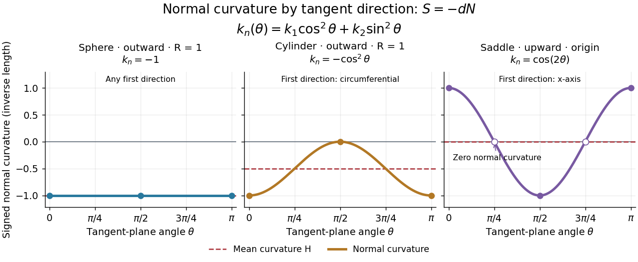
Each graph uses angle $\theta$ in the tangent plane, measured from the indicated first principal direction. The sphere and circular cylinder have $R=1$; the saddle graph refers only to the origin. Reversing the unit normal reflects each normal curvature graph through zero, negates both principal curvatures and the mean curvature, and preserves their product, the Gaussian curvature.

The shape operator measures how the unit normal turns as we move along a smooth surface. A plane has a constant unit normal, whereas the outward unit normal of a sphere turns in every direction in the tangent plane. Keeping the direction of this change, rather than just its magnitude, lets one recover the principal curvatures and their principal directions.

Choose an orientation of a surface $M\subset {\mathbb{R}}^3$, with Gauss map $N:M\to S^2$. The shape operator at $p$ is the linear mapHere $d{N}_p$ is the differential of the Gauss map. Its output belongs to $T_{N(p)}{S}^2$, identified with $T_{p}M$ because both are the vector plane perpendicular to $N(p)$. The minus sign is our convention throughout this branch. ^[ref]

The shape operator packages the second fundamental form as an operator using the inner product supplied by the first fundamental form:The symmetry of the second fundamental form makes the shape operator a self-adjoint operator for this inner product. Thus an orthonormal basis of principal directions diagonalizes it. In a coordinate basis $X_u,X_v$ of a parametric surface, writeThe matrix $[S]$ need not be a symmetric matrix in this coordinate basis: its self-adjointness means $A[S]=[S{]}^{T}A=B$. Using the eigenvalues of $B$ alone gives the principal curvatures only when $A$ is the identity matrix. ^[ref]

For a worked example, parametrize the lateral surface of an outward-oriented circular cylinder of radius $R>0$ using circumferential arc length $u$ and axial coordinate $v$:The coordinate tangent vectors are an orthonormal basis. Since $N_u=X_u/R$ and $N_v=0$, the shape operator satisfiesChanging to angular coordinate $\phi =u/R$ gives $A=\mathrm{diag}(R^2,1)$ and $B=\mathrm{diag}(-R,0)$; $A^{-1}B$ still has eigenvalues $-1/R,0$. This is why the first fundamental form must participate in the calculation.

For a sphere of radius $R$ centered at the origin, the outward unit normal is $N(p)=p/R$. Hence $S_{p}v=-v/R$, so both principal curvatures are $-1/R$. For a plane, $dN=0$ and the shape operator vanishes. Reversing the unit normal negates the shape operator and both principal curvatures; the Gaussian curvature remains unchanged while the mean curvature changes sign, as in orientation reversal of surface curvature.

For a nondegenerate convex minor spherical triangle, the spherical law of cosines relates two angular sides $b,c$, their included interior angle $A$, and the opposite angular side $a$:Relabelling the vertices gives the corresponding formulas for $b,B$ and $c,C$. As with the spherical law of sines, physical side lengths must first be divided by the sphere's radius. The spherical law of cosines determines $a\in (0,\pi )$ uniquely from $b,c,A$ when the data describe such a spherical triangle. It also recovers each interior angle from three sides, for exampleUsing the cosine and the range $0<A<\pi$ selects a unique angle, avoiding the supplementary-angle ambiguity of an inverse sine calculation.

To derive the spherical law of cosines, let $u,v,w$ be the vertex unit vectors at $A,B,C$, so $u\cdot v=\cos c$, $u\cdot w=\cos b$ and $v\cdot w=\cos a$. The outgoing unit tangent vectors at $u$ are $t_B=(v-\cos cu)/\sin c$ and $t_C=(w-\cos bu)/\sin b$. Their dot product is both $\cos A$ and $(\cos a-\cos b\cos c)/(\sin b\sin c)$, proving the identity. This gives a geometric explanation: spherical trigonometry compares angles in the tangent plane using vectors in the surrounding Euclidean space.

For a worked example on the unit sphere, take the verticesAt $A$, the outgoing unit tangent vectors are $(1,0,0)$ and $(0,1,0)$, so the interior angle is a right angle. The vertex dot products give $b=c=\pi /3=60^{\circ }$. The spherical law of cosines then reduces to the right-angle identity $\cos a=\cos b\cos c$, givingTo find $B$, use the relabelled spherical law of cosines:The physical side lengths on a sphere of radius $R$ are ${\ell }_a\approx 1.318116R$ and ${\ell }_b={\ell }_c=\pi R/3\approx 1.047198R$. For example, on a toy sphere with $R=10$ metres they are approximately $13.18116$, $10.47198$ and $10.47198$ metres; the interior angles stay the same. Applying the planar Pythagorean theorem directly to the angular sides would instead give $\sqrt{60^2+60^2}\approx 84.852814^{\circ }$. That flat right triangle calculation does not give the great-circle distance between $B$ and $C$.

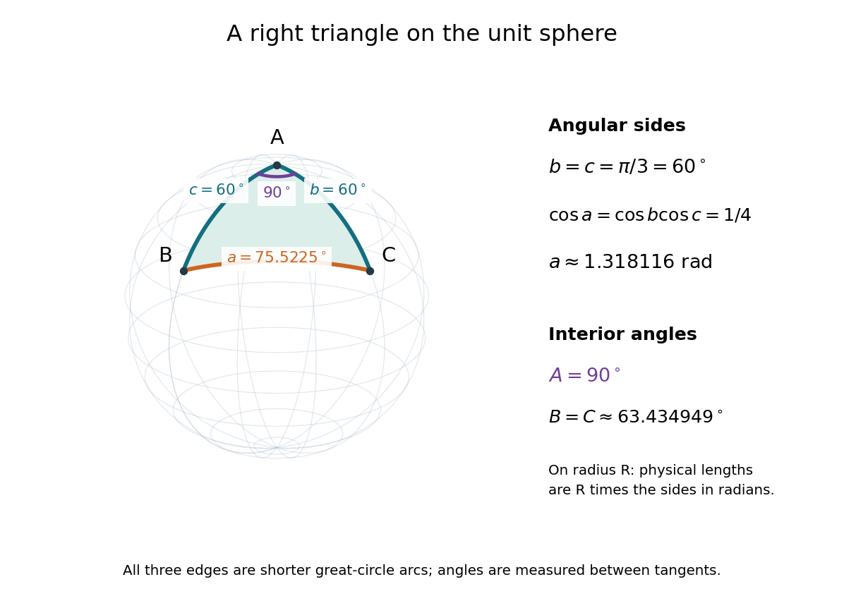
The familiar law of cosines reappears as a local approximation. With $a,b,c$ all small in radians, substitute the small-angle approximations $\sin x\approx x$ and $\cos x\approx 1-x^2/2$ into the spherical law of cosines and keep terms through second order:Multiplication by $R^2$ gives the planar law of cosines for the physical side lengths. For a fixed small surface triangle on a progressively larger sphere, the angular sides shrink and this approximation improves. Thus the curved and flat formulas fit together: the Pythagorean theorem is recovered locally when $A$ is a right angle.

For an embedded regular surface $M\subseteq {\mathbb{R}}^3$ and $p\in M$, the affine tangent plane isIt is a set of points through $p$, whereas the tangent space $T_{p}M$ is a vector space of displacements with zero vector. Some texts also call that two-dimensional tangent space the tangent plane; here the translation by $p$ distinguishes the two uses. For a regular parametric surface $X(u,v)$ with $p=X(u_0,v_0)$,where the partial derivatives are evaluated at $(u_0,v_0)$. Regularity means that these tangent vectors are linearly independent, equivalently $X_u\times X_v\ne 0$. Their cross product is a normal vector. ^[ref]

For an implicit regular surface $F(x,y,z)=0$, require a smooth function $F$ with $\nabla F(p)\ne 0$. ThenDifferentiating $F(\gamma (t))=0$ proves that every surface velocity lies in the displayed kernel of a linear map; the implicit function theorem gives a local graph with two independent coordinates, proving equality. The gradient is the normal vector with respect to the ambient dot product. ^[ref]

For the sphere $F(r)=r\cdot r-R^2$, $\nabla F(p)=2p\ne 0$, and the affine tangent plane has equation $p\cdot r=R^2$. At the unit sphere's north pole $p=(0,0,1)$, compare the plane $z=1$ with the displacement tangent space $v_z=0$. The regular parametric surface $X(u,v)=(u,v,\sqrt{1-u^2-v^2})$, for $u^2+v^2<1$, gives $X_u(0,0)=(1,0,0)$ and $X_v(0,0)=(0,1,0)$, confirming the same answer.

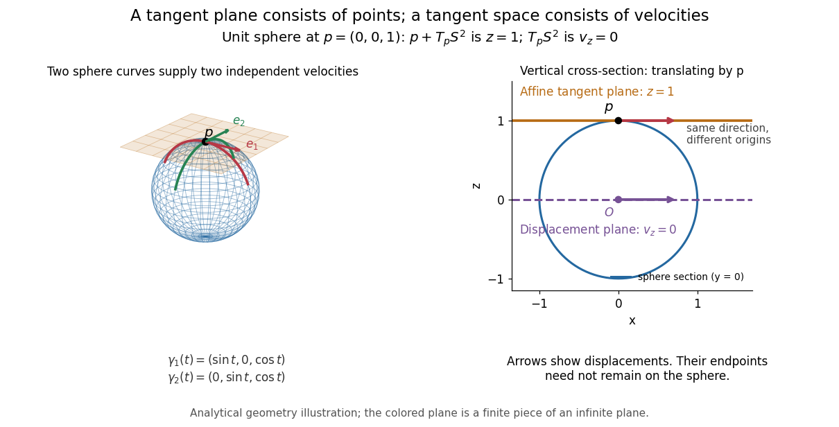
This analytical illustration shows a unit sphere and a vertical cross-section. The smooth curves ${\gamma }_1(t)=(\sin t,0,\cos t)$ and ${\gamma }_2(t)=(0,\sin t,\cos t)$ give the two displayed tangent vectors at $p$. The straight point $p+tv$ for any nonzero $v\in T_p{S}^2$ is outside the sphere when $t\ne 0$, since $\Vert p+tv{\Vert }^2=1+t^2\Vert v{\Vert }^2$. A tangent plane therefore captures first-order motion, not an exact patch of the regular surface.

The same idea makes local approximation useful. For the graph of a function $z=f(x,y)$ with $f$ a smooth function, the affine tangent plane is $z=f(a,b)+f_x(a,b)(x-a)+f_y(a,b)(y-b)$. ^[ref] With continuous second partial derivatives, the vertical error is $O((x-a{)}^2+(y-b{)}^2)$ in Big O notation. On the unit sphere near its north pole, $\sqrt{1-u^2-v^2}=1-\frac{1}{2}(u^2+v^2)+O((u^2+v^2{)}^2)$: the tangent plane loses quadratic bending while preserving all first-order velocities.

A failed regularity test needs interpretation. Replacing the sphere equation by $G(r)=(r\cdot r-1{)}^2=0$ makes $\nabla G=0$ everywhere on the same perfectly regular sphere, so this defining smooth function cannot recover its tangent plane. Similarly, the usual spherical parametric surface loses matrix rank at the poles, while the graph parametrization above remains regular there. A vanishing gradient or degenerate parametrization invalidates that calculation; it alone does not prove that the underlying geometry has no tangent plane.