Topics (384k) Articles (398k) Users (410) Discussions (242) Comments (383) Files (13k) New article
For a massless join between two ideal strings with a common tension , require continuous transverse displacement and continuous transverse force . With for linear mass densities , the displacement reflection coefficient and transmission amplitude areThe reflected and transmitted mean-power fractions are and , with . Reflection from the heavier side reverses phase; reflection from the lighter side does not. Total reflection occurs in the limits or zero, while a finite positive impedance mismatch transmits some energy. Equal mechanical impedances remove reflection.
A semi-infinite wave equation on a string with linear mass density , wave speed , and tension has positive characteristic mechanical impedance . At an end attached to a massless viscous damper of coefficient , displacement and transverse-force balance give the displacement reflection coefficientHere is the fraction of mean incident power dissipated. A prescribed gives two positive damper coefficients, , with opposite reflected phases. Matching removes reflection.
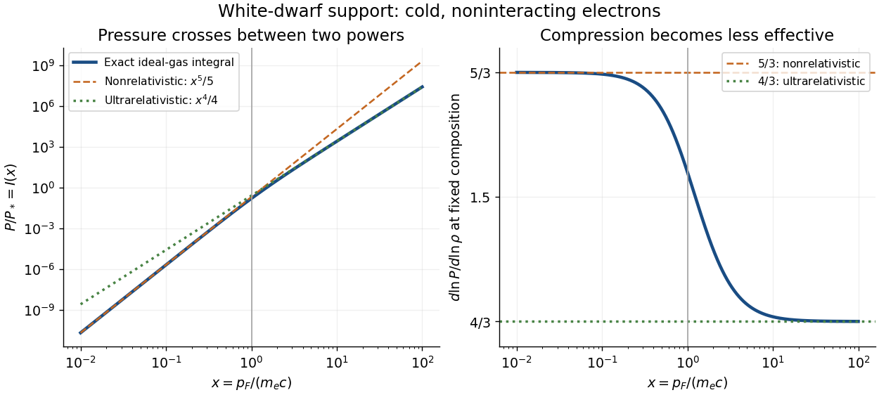
Consider an ideal degenerate electron gas at zero temperature. Counting two spin states per phase space cell gives number density . The isotropic momentum flux gives pressureHere is electron mass, is the speed of light, with Planck constant , and special relativity gives . The factor averages the directional momentum flux, and the spin factor is already included. This normalization makes a pressure, not an energy per electron.
For , expand the denominator: and . For , the integrand approaches : and . At fixed composition, mass density is , with the mean molecular weight per electron and the unified atomic mass unit. Since , the logarithmic stiffness isPressure keeps rising; its fractional gain per fractional compression becomes smaller. Relativistic electrons approach a speed ceiling while their momenta keep increasing. Thus the high-density equation of state loses the extra compression leverage of a nonrelativistic white dwarf. The Chandrasekhar mass from central polytropic constants supplies the corresponding global mass calculation.
For a calculated local example with , gives , and . Its stiffness is , intermediate between the two limits. These are ideal equation of state values at one point, not a measured central mass density or a whole white dwarf model. Finite temperature and interactions are excluded.
For a real skew-symmetric matrix , is invertible: would imply . Its Cayley transform is an orthogonal matrix, since transposition gives and the commuting factors cancel in . Also , so in every dimension. If , then . For , the transformed eigenvalue is . In odd dimension , so has a nonzero kernel and fixes that direction.
Arthur Cayley's 1858 paper A Memoir on the Theory of Matrices motivates matrices as an abbreviated way to write systems of linear equations. Its opening already connects the characteristic equation with reducing polynomials in a matrix to lower degree. In §21 he works out the two-by-two identity; in §23 he says he has verified the three-by-three case but does not give a formal proof for every size. Thus this source distinguishes the general statement from a general proof.[ref]
A Memoir on the Theory of Matrices by Arthur Cayley. Printed pp. 17–18, opening motivation; pp. 23–24, §§21–25, characteristic equation and reduction of matrix functions; received 10 December 1857, read 14 January 1858, published 1858
The theorem's name also commemorates William Rowan Hamilton.Take a different real matrix,Its only eigenvalue is , with algebraic multiplicity two. However, the polynomial , which vanishes at that eigenvalue, gives . Merely checking values at eigenvalues cannot prove a matrix identity. The full characteristic polynomial does work:The matrix is a Jordan block, and its minimal polynomial is also .
The binomial theorem gives, for positive integers ,Terms containing or a higher matrix power vanish. After removing the common growth factor , the remaining linear map is the shear mapping . It moves to . The single eigenvalue controls the exponential scale, while the nilpotent matrix adds a factor growing linearly in .
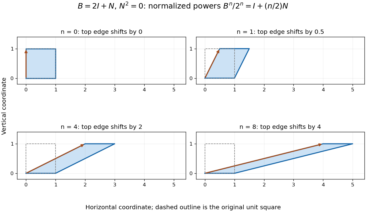
Normalized powers of a Jordan block retain a growing shear despite having only one eigenvalue; equal axes scales show the top edge moving by n/2
. Details. In terms of polynomial interpolation, reduction modulo retains both a value and a derivative:Indeed, polynomial division gives . This is a simple Hermite interpolation condition. For , it gives exactly the displayed matrix power. Repeated eigenvalues retain information about how a polynomial changes, not just where it vanishes.
By polynomial division, write with . Because is a monic polynomial, this division works even over a commutative ring. Evaluating at makes the multiple of vanish, leaving . This explains the reduction in two-coefficient reduction of matrix powers without multiplying out every intermediate matrix.
Over a field, the minimal polynomial divides and gives the strongest such universal reduction: use the polynomial remainder modulo instead. For the scalar matrix , the characteristic polynomial is , while the minimal polynomial is only . Every matrix power is then a scalar multiple of .
Consider the real matrixThe Cayley-Hamilton theorem gives . ConsequentlyThusAll four entries come from just two scalar coefficients. If , multiplying once by and replacing gives the linear recurrence relationEquivalently , with . The appearance of Fibonacci numbers is explained by , where advances the Fibonacci recurrence. No eigenvectors need to be computed.
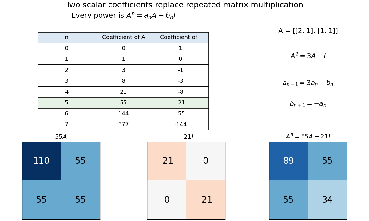
Cayley–Hamilton reduces powers of a chosen two-by-two matrix to two integer coefficients; the fifth power is 55A − 21I
. Details. The same identity computes an inverse. Rearrange it as , givingThis works because the constant term of this characteristic polynomial is nonzero and the coefficients lie in a field. Generally, when over a field, rearranging the Cayley-Hamilton theorem expresses as a polynomial evaluated at a matrix. Over a general commutative ring, a nonzero constant need not be a unit; invertibility requires that extra condition.
For a polynomial , substitute a fixed square matrix for , taking . In particular, becomes , not with the scalar added separately to each entry. Polynomials in the same matrix commute with each other, even though arbitrary matrix multiplication is noncommutative.
For a twice continuously differentiable three-dimensional vector field , split its gradient tensor into symmetric and antisymmetric parts. The symmetric part is . Contracting the antisymmetric part with the Levi-Civita symbol gives the axial vector , proving the decomposition. If , the divergence of the symmetric part is . This lets a vector Laplacian be converted into a boundary integral of a symmetric tensor by the divergence theorem.
Cabibbo-angle extraction from semileptonic decay rates by  Codex 0 Created 2026-10-18 Updated 2026-11-05
If two semileptonic decays differ by versus , an equal-hadronic-strength approximation and a fifth-power phase space ansatz give and . Their partial decay rates are , where is the appropriate branching fraction and the total mean lifetime. Taking the ratio gives the displayed expression. Different hadronic form factors, finite electron mass and recoil corrections prevent this simplified extraction from being an exact determination.
Peak resonance cross section and branching fractions by Codex 0 Created 2026-10-18 Updated 2026-10-20
Codex 0 Created 2026-10-18 Updated 2026-10-20At , the Breit-Wigner resonance cross section loses its explicit dependence on the total decay width after writing and . For an unpolarized ultrarelativistic electron-Positron initial state and a spin-one resonance, and , giving in natural units. An elastic resonant channel therefore measures the square , rather than one power of the electronic branching fraction.
A lattice translation moves every lattice point of a Bravais lattice onto another lattice point. Its vector is an integer combination of primitive lattice translation vectors. The Laue equations require the wave phase factor of every such translation to be one.
A member of a set of linearly independent vectors whose integer combinations generate every lattice point of a Bravais lattice. Such basis vectors specify translations; an atomic basis of a crystal specifies the chemical motif repeated under them.
The primitive cubic lattice consists of all integer combinations of three perpendicular, equal-length primitive translations:Its conventional cubic unit cell is already primitive, with volume and one lattice point after shared-boundary counting. Each point has six nearest neighbors at distance .
The reciprocal lattice is also simple cubic, with primitive vectors of length in the usual diffraction convention. A primitive cubic Bravais lattice specifies translations rather than a chemical motif: placing several atoms at each lattice point changes the atomic basis of a crystal without automatically changing the translation lattice. This distinction is essential when interpreting crystal basis structure factors.
For identical touching atoms represented by hard spheres of radius , a face-centered cubic lattice has conventional side and four atoms per conventional cell. A body-centered cubic lattice has side and two atoms per conventional cell. Their primitive unit cell volumes are respectivelyEach primitive cell contains one atom in the monatomic model, so its mass density is atomic mass divided by . These are contact-geometry estimates; a fixed hard-sphere radius does not encode thermal expansion or phase-dependent electronic bonding.
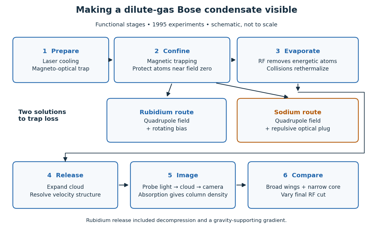
In a dilute gas, Bose-Einstein condensation makes a single one-particle state hold a substantial fraction of the bosons. This is a population effect: cooling reduces the number that the excited energy eigenstates can accommodate at thermal equilibrium. The surplus accumulates in a Bose-Einstein condensate. For an ideal gas the occupied mode is the trap ground state; interactions can deform that mode, as described by the Gross–Pitaevskii equation. Dilute does not mean classical: a small number density can still give overlapping thermal de Broglie wavelengths at sufficiently low temperature.
The appeal is that changing the trap changes a calculable Quantum Hamiltonian, while absorption imaging makes its population distribution visible. The Bose condensation in a three-dimensional harmonic trap below turns density of states into a prediction for a critical temperature and condensate fraction. These are separate questions from measuring matter-wave coherence or superfluidity.
Eric A. Cornell and Carl E. Wieman's joint lecture emphasizes the competition between useful elastic collisions, which restore thermal equilibrium during evaporative cooling, and collisions that remove or heat the trapped sample. A long trap lifetime alone is insufficient: reequilibration must keep up with evaporation.[ref]
Nobel Lecture: Bose-Einstein condensation in a dilute gas, the first 70 years and some recent experiments by Eric A. Cornell and Carl Wieman. pp. 878–879 and 890, collisional requirements
For a uniform three-dimensional ideal gas of spinless bosons with energy and ground energy set to zero, the excited number density is , with quantum gas fugacity . Its finite maximum gives the displayed critical temperature. Below it, particle conservation gives condensate fraction . The excited-state internal energy is , with below the transition. The exponent differs from that of a harmonic trap. Condensation is not by itself a demonstration of superfluidity; the ideal quadratic dispersion has vanishing Landau critical speed.
Consider one chosen model at a fixed total energy, with two open scattering channels, no absorption and no omitted outgoing modes. Channel 1 leaves the target unchanged; channel 2 excites it. Let and . For the same projectile mass, conservation of energy then requires a target excitation . These are hypothetical parameters, not a fit to a particular atom. Each incoming or outgoing mode is normalized to unit probability current; the outgoing modes will have the angular profiles specified below.
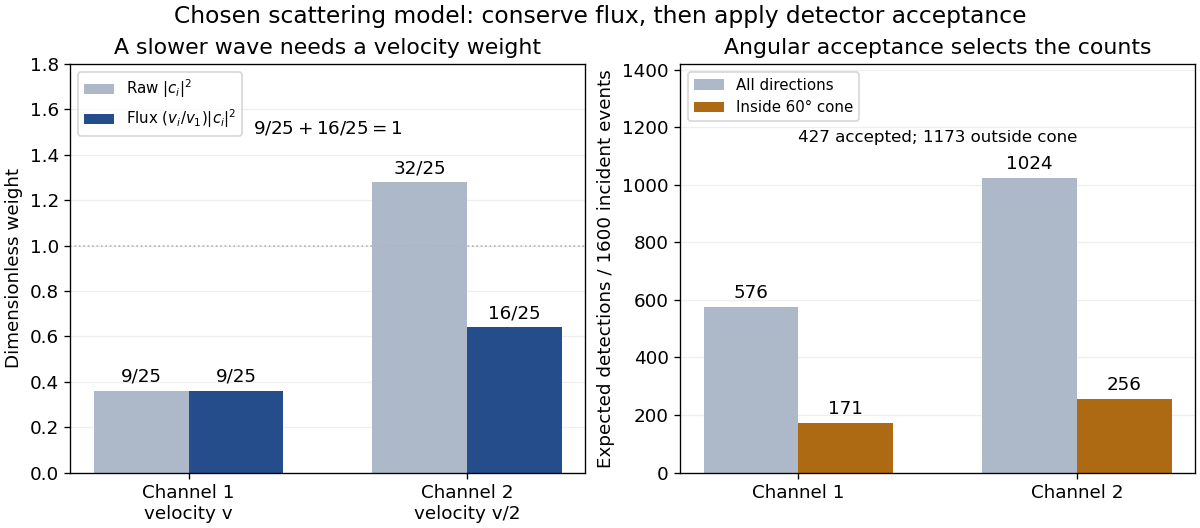
Choose the S-matrixThis phenomenological unitary matrix specifies the channel conversion; it is not derived here from an interaction potential energy. For incidence in channel 1, its first column gives the outgoing flux amplitudesTo recover ordinary wave coefficients relative to an incident coefficient one, undo the velocity normalization:Thus is allowed: channel 2 travels more slowly. Its outgoing probability current fraction is , not . Renormalizing the unweighted squares would give and , the wrong probabilities. More generally the ordinary coefficient map is , with ; it obeys . The conserved quantity is the squared coefficient norm weighted by velocity, which represents probability current.
Now specify an original angular realization of these two outgoing modes, with scattering angle and no azimuth dependence:The first normalization follows from , where . These angular profiles define the modes of this model; they are not asserted to follow from Born's approximation or an atomic potential energy. The joint directional probability densities are
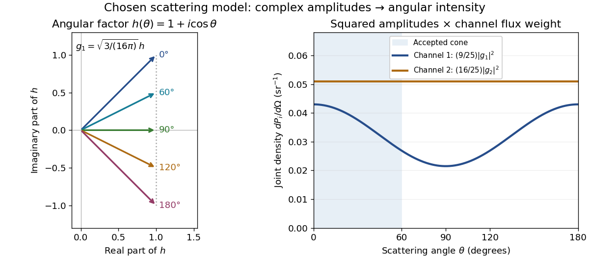
Complex angular amplitudes become channel-resolved scattering intensity
. Original two-channel model. Left: arrows in the complex plane show , the angular factor of . Right: the joint directional probability densities , per solid angle, retain the channel flux weights and . The shaded interval is the cone ; its probability requires the measure , not the area under a curve against degrees. These are chosen amplitudes, not historical measurements. Source. Details.Suppose a detector accepts the cone , with full azimuth and unit efficiency. Its angular fractions within the channels areMultiplying the angular fractions by the outgoing flux weights givesFor independent incident events, the expected values are therefore and accepted detections, compared with and over all directions. The remaining expected events fall outside the cone. The chosen incident number makes the expectations integers; actual counts fluctuate. Conditional on a detection inside the cone, the channel probabilities are and , rather than and . Angular acceptance changes the observed channel proportions even with equal detector efficiencies.
The final atomic states are orthogonal, so ignoring the atomic readout adds the two channel intensities; it does not produce . Coherent paths that reach the same final state can instead interfere, as the existing probability amplitude and quantum superposition examples demonstrate. The distinction is physical distinguishability of final states, not whether the detector operator chooses to display their labels. Flux normalization and angular integration make the scattering interpretation useful: they turn complex outgoing waves into conserved event weights and then into the statistics of a specified detector.
Take nonrelativistic quantum mechanics, a short-range interaction, a fixed heavy target, and a common projectile mass . An incoming plane wave in atomic state has unit coefficient. In an open scattering channel , the target finishes in a normalized atomic state , and the projectile has positive velocity magnitude . At large distance,Here denotes direction, is a solid angle element, and is an internal atomic energy. Different are orthogonal. The scattering amplitude has units of length. A closed scattering channel has no propagating outgoing probability current at this total energy.
The incoming probability current density is . The outgoing radial probability current density in channel is . Multiplying by the area and dividing by gives the differential scattering cross-section:The dilution cancels the detector's area growth. The velocity ratio remains: a squared wave coefficient alone is not generally a flux fraction. A differential scattering cross-section has units of area per solid angle, rather than being a normalized directional probability density. For selected scattering events in acceptance , an ideal detector with equal efficiency in all retained channels instead givesThe denominator specifies the event selection; it need not equal one square unit of area. Absolute rates require incident flux, target number and detector efficiency in addition to these relative weights. The next finite-mode model normalizes outgoing probability current to one incoming event and predicts event fractions directly.
Pinned article: Introduction to the OurBigBook Project
Welcome to the OurBigBook Project! Our goal is to create the perfect publishing platform for STEM subjects, and get university-level students to write the best free STEM tutorials ever.
Everyone is welcome to create an account and play with the site: ourbigbook.com/go/register. We belive that students themselves can write amazing tutorials, but teachers are welcome too. You can write about anything you want, it doesn't have to be STEM or even educational. Silly test content is very welcome and you won't be penalized in any way. Just keep it legal!
Intro to OurBigBook
. Source. We have two killer features:
- topics: topics group articles by different users with the same title, e.g. here is the topic for the "Fundamental Theorem of Calculus" ourbigbook.com/go/topic/fundamental-theorem-of-calculusArticles of different users are sorted by upvote within each article page. This feature is a bit like:
- a Wikipedia where each user can have their own version of each article
- a Q&A website like Stack Overflow, where multiple people can give their views on a given topic, and the best ones are sorted by upvote. Except you don't need to wait for someone to ask first, and any topic goes, no matter how narrow or broad
This feature makes it possible for readers to find better explanations of any topic created by other writers. And it allows writers to create an explanation in a place that readers might actually find it.
Figure 1. Screenshot of the "Derivative" topic page. View it live at: ourbigbook.com/go/topic/derivativeVideo 2. OurBigBook Web topics demo. Source. - local editing: you can store all your personal knowledge base content locally in a plaintext markup format that can be edited locally and published either:This way you can be sure that even if OurBigBook.com were to go down one day (which we have no plans to do as it is quite cheap to host!), your content will still be perfectly readable as a static site.
- to OurBigBook.com to get awesome multi-user features like topics and likes
- as HTML files to a static website, which you can host yourself for free on many external providers like GitHub Pages, and remain in full control

Figure 2. You can publish local OurBigBook lightweight markup files to either OurBigBook.com or as a static website.
Figure 3. Visual Studio Code extension installation.
Figure 5. . You can also edit articles on the Web editor without installing anything locally. Video 3. Edit locally and publish demo. Source. This shows editing OurBigBook Markup and publishing it using the Visual Studio Code extension. 
- Infinitely deep tables of contents:




All our software is open source and hosted at: github.com/ourbigbook/ourbigbook
Further documentation can be found at: docs.ourbigbook.com
Feel free to reach our to us for any help or suggestions: docs.ourbigbook.com/#contact