
Subduction zone segmentation is the observation that slab structure, fault slip and upper-plate behavior change along a margin; their boundaries need not coincide exactly. In Cascadia, it is documented by several independent measurements.
Onshore GNSS velocities, coastal leveling and tide gauges constrain along-strike changes in megathrust locking and interseismic uplift. Episodic tremor and slip has distinct recurrence and migration patterns, and its occurrence is lower in parts of central Oregon than farther north and south. Coastal geological records constrain differences in coseismic subsidence and the extents of past ruptures. Those observations sample different depths and time windows, so a present-day locking boundary should not automatically be declared a permanent earthquake rupture barrier. A 2014 analysis found persistent central-margin partial creep compatible with reduced uplift, reduced paleoseismic subsidence and lower cumulative slow slip.[ref]
Central Cascadia subduction zone creep by Gina M. Schmalzle and others. Conclusions, central Cascadia approximately 43–46°N and comparison of GPS, uplift and paleoseismic observations
A physically specific hypothesis links these variations to subslab mantle buoyancy. An onshore–offshore seismic tomography study imaged low-velocity asthenosphere beneath northern and southern Cascadia, spatially associated with stronger plate locking and more tremor, with different central-margin structure. Warmer or partly molten asthenosphere can be less dense. Its buoyant traction can push upward against the slab and change contact stresses on the megathrust. Hotspot-influenced material is one proposed northern source; three-dimensional deformation near the Gorda region offers a southern upwelling mechanism.[ref]
Buoyant Asthenosphere Beneath Cascadia Influences Megathrust Segmentation by Miles Bodmer and others. Abstract; sections 3 and 4, onshore–offshore tomography and proposed northern/southern buoyancy sources
There are additional controls. The Siletzia basaltic basement beneath the overriding plate varies in extent and thickness. Its permeability and stiffness can affect fluid escape and fault stresses: poorly drained material can preserve high pore pressure, lower effective normal stress and promote creep. Along-strike changes in incoming plate age, slab dip, fracture-zone hydration, sediment supply and plate-edge stresses can also modify the thermal and frictional environment. Central-margin creep has specifically been associated with the distribution of Siletzia and inferred fluid trapping.[ref]
Central Cascadia subduction zone creep by Gina M. Schmalzle and others. Discussion and conclusions, Siletzia gravity signature and the permeability/fluid-pressure interpretation
How do we distinguish these causes? Offshore and onshore seismic arrays test the geometry of the anomalies; resolution and synthetic-recovery tests determine whether apparent segmentation could result from uneven station coverage. Seismic attenuation, anisotropy, magnetotelluric sounding, rock physics and heat-flow data help separate temperature, melt, water and composition. Gravity anomalies and seismic interfaces constrain basement and slab geometry; geodetic inversions test whether the inferred locking pattern persists across plausible fault geometries. Forward models then ask whether the measured density or pore-pressure contrasts produce stresses and slip patterns of the required size and sign.
Segmentation is observed robustly; a unique cause is not established by spatial correlation alone. Seismic velocity is not a direct density measurement, central creep and deep tremor are not the same phenomenon, and multiple coupled structures can reinforce one another. The buoyant-mantle and upper-plate fluid hypotheses are testable explanations rather than mutually exclusive certainties.
The positive centers in the supplied maps are examples of lunar mascons, especially associated with large impact basins. An empty excavation by itself removes mass and would not explain a positive central anomaly. Basin formation can thin the low-density lunar crust and raise denser lunar mantle beneath the floor; impact melting, collapse and later cooling can also create dense material and lock in a mass excess. Where a basin was later flooded, dense mare basalt adds another contribution. Mare infill is therefore one possible contributor, not a necessary explanation of every mascon.[ref]
NASA's GRAIL Mission Solves Mystery of Moon's Surface Gravity by National Aeronautics and Space Administration. Mission-team account of impact excavation, collapse, cooling and the central mass excess, 30 May 2013
The difference between the maps is the modeled topographic contribution. On a common reference surface, write schematicallyThe free-air gravity anomaly retains relief-related attraction. Rims, excavated floors and central peaks therefore contribute fine structure. The Bouguer gravity anomaly removes the attraction predicted from the measured topography at an assumed crustal density, making internal density and interface structure more apparent. A low basin floor has a negative topographic contribution; subtracting it can enhance an underlying positive central anomaly. Removing a positive rim contribution can weaken a rim high. The supplied lower map is correspondingly smoother at short wavelengths and shows prominent residual basin centers and surrounding rings. This is a change of gravity reduction, not a physical change of the craters.[ref]
GRGM900C: A degree 900 lunar gravity model from GRAIL primary and extended mission data by Frank G. Lemoine and others. Sections 4.2–4.3, gravity predicted from topography and its subtraction to obtain Bouguer gravity
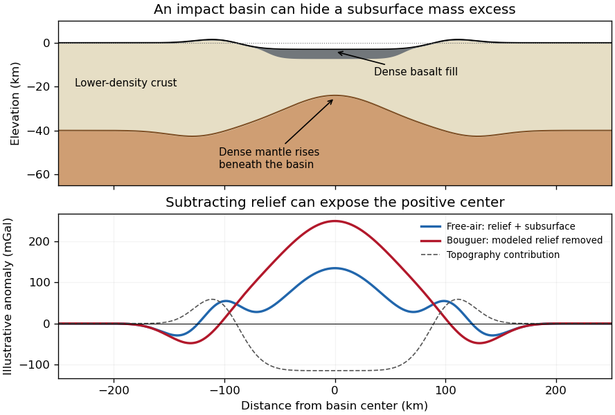
Original schematic showing how dense fill and mantle uplift can outweigh an excavated basin's missing surface mass; illustrative curves are not GRAIL measurements
. Details. For scale, a Bouguer slab approximation gives . A km layer with geophysical density contrast produces about mGal above an ideal infinite slab. Actual basin geometry, burial, porosity and mantle uplift require a finite three-dimensional model. Smaller craters can have central lows, damaged porous interiors or more complex rings; the maps do not imply that every crater has a positive anomaly or that positive anomalies measure basalt thickness uniquely.
I would test whether the ancient farside crust grew locally with an early thermal/compositional gradient or acquired a substantial later accreted layer. The research programme should estimate a globally consistent crustal mass and chronology before tuning either mechanism to a single attractive map.
First, map crustal geometry with independent density constraints. Jointly invert GRAIL gravity and laser-altimeter surface topography, allowing spatially varying density and porosity rather than converting every anomaly to thickness. A new broad-band seismic network should include farside stations, long-lived polar power systems and a communications relay. Natural impacts and moonquakes, supplemented by calibrated active sources near landing sites, would constrain layer velocities, attenuation, crustal interfaces and the crust-mantle boundary. Crossing ray paths and receiver-side conversions are essential to distinguish a thick crust from an incorrect density or velocity assumption. A coherent buried layer or age-correlated discontinuity across the farside would favor addition or stacking; a gradual hemispheric compositional gradient would better support asymmetric local growth. Neither pattern is guaranteed to survive later impacts.
Second, obtain samples that address the initial contrast. Collect geographically distributed ancient highland rocks from both hemispheres, using basin ejecta, central peaks and drilling to sample beneath the impact-gardened regolith. Return samples with mapped geological context. Mineral chemistry and bulk Ca–Al–Mg–Fe abundances would test a primary refractory gradient; crystallization ages would date crustal construction, while shock-reset ages would date overprinting. Isotopic and trace-element measurements could identify an accreted population, but similar isotopes are possible for material derived from the same early debris system. A young deposit draped over older crust would favor accretion; coeval flotation-related crust with a systematic chemical gradient would favor local asymmetric differentiation. Multiple sites are necessary because a single basin's ejecta can mix distant sources.
Third, measure the thermal and volcanic consequences. Place shielded, sufficiently deep heat flow probes in representative highlands and mare terrains. Combine their geothermal gradients and measured thermal conductivity with orbital gamma-ray constraints on heat-producing elements. Map mare volumes and eruption ages, rather than only their exposed areas, to separate melt production from storage and eruption efficiency. A strong correlation between late volcanism, subsurface heat producers and high inferred mantle temperatures would support radiogenic amplification, while old crustal asymmetry without that correlation would show that later heating is not the entire cause.
Finally, compare forward models against withheld observations. Couple irradiation, vapor transport, condensation, lunar magma ocean mixing and crystallization for the thermal scenario; couple orbital evolution, impact deposition, mixing and later viscous relaxation for accretion. Account for later true polar wander before treating present-day hemispheric orientation as the original formation geometry. Require each model to conserve mass and energy and to reproduce the independent thickness, chemistry, age and volcanic data within their uncertainties. Vary unknown initial conditions and compare predicted observables at sites not used for calibration. The discriminating outcome is a conjunction such as a coherent accreted unit with a consistent emplacement age, or an ancient chemical gradient quantitatively consistent with transport under Earth irradiation. A lower gravity misfit alone cannot establish the historical mechanism, because gravity is a nonunique inverse problem.
The lunar crustal dichotomy combines several observables: the far side of the Moon has generally thicker, higher, feldspathic lunar highlands, whereas most visible lunar maria and the Procellarum KREEP Terrane occupy the near side of the Moon. These need not all have been produced by a single event. The old anorthosite crust formed mainly before the younger basaltic mare infill. Gravity-based crustal models combined with sample and seismic constraints demonstrate that crustal thickness and porosity must be considered alongside surface color.[ref]
The Crust of the Moon as Seen by GRAIL by Mark A. Wieczorek and colleagues. Science 339, p. 671, crustal density, porosity and thickness constraints
An early thermal and chemical asymmetry is one physically motivated option. In a lunar magma ocean, crystallizing, relatively buoyant plagioclase can accumulate to form feldspathic crust. On a young Moon that rapidly attained synchronous rotation, radiation from a still-hot nearby Earth would preferentially warm the nearside. The primordial Earthshine hypothesis proposes that this imposed a thermal gradient in the atmosphere and accreting material: crust-forming refractory constituents condensed preferentially toward the cooler farside, favoring thicker farside crust. This is more specific than simply saying that the farside cooled faster; it requires a persistent hemispheric chemical contrast.[ref]
Earthshine on a Young Moon: Explaining the Lunar Farside Highlands by Arpita Roy and others. Sections 2–4, early tidal locking, condensation gradient and survival of compositional asymmetry
Subsequent concentration of incompatible elements in KREEP-rich late liquids can help preserve a thermal asymmetry: potassium, uranium and thorium provide radiogenic heating, supporting later melting in the nearside source region. Lower surface elevation and a thinner crust also facilitate some magma transport and pooling, although crustal thickness alone cannot specify eruption rates. The origin of the crustal contrast and the later production and emplacement of mare basalt are separate parts of the explanation.
The thermal option is consistent with a thick feldspathic farside crust, a hemispheric chemical contrast and the existence of an early hot Earth. It is not uniquely demonstrated by those observations. Vigorous magma-ocean mixing could erase the proposed gradient; the required irradiation must persist during the relevant condensation and crust-building interval, not merely occur at some early time. A failure to find the predicted bulk compositional contrast in demonstrably ancient deep crust, or a chronology placing the asymmetry after complete crystallization, would challenge this particular mechanism. The existence of farside mare deposits and large thin-crust basins also warns against treating thickness as an on/off volcanic switch.
Accretion of a smaller companion is a contrasting option. A low-speed collision of a smaller co-orbiting moon with the lunar farside could add a broad layer of relatively cold silicate material rather than excavate an ordinary deep crater. Numerical impact models demonstrate that such a depositional event can build thick highlands and displace underlying residual liquid toward the opposite hemisphere.[ref]
Forming the lunar farside highlands by accretion of a companion moon by Martin Jutzi and others. Nature 476, pp. 69–72, accretionary collision model
Broad crustal excess and asymmetric evolved material are compatible with that mechanism, but are not unique evidence for it. The necessary companion, collision timing and impact geometry must be dynamically feasible. A predicted buried depositional interface, age discontinuity or lateral fabric should survive somewhere; their systematic absence in well-resolved, unmodified ancient crust would count against the model. Closely related bodies could have similar isotopes, so failure to find a large isotopic difference alone would not disprove accretion.Both scenarios allow later basin impacts, partial melting of the lunar mantle and mare emplacement to modify the original contrast. A useful explanation must reproduce crustal mass, chemistry, chronology and volcanic distribution together, and state which observations would distinguish its initial cause.
The geological record is a collection of thermometers with different sampling biases, not a direct time series of the whole mantle.
Primary melt compositions constrain melting temperatures. Reconstruct primary magma compositions from dated, suitably unaltered basalts by correcting for fractional crystallization and checking equilibrium with olivine. Experimental phase equilibrium constraints and mineral–melt thermometers then constrain the pressure and temperature of melt generation. In laboratory calibrations, a candidate melt and mineral assemblage are equilibrated at controlled pressure and temperature, quenched, and their crystals and glass analyzed. Repetition across adjacent conditions brackets the relevant phase equilibrium boundaries. Correcting for decompression and latent heat then allows comparison as mantle potential temperature. Age-controlled, non-arc basalt suites are especially valuable for separating changes in ambient mantle from exceptional mantle plumes. The 2010 reconstruction by Claude Herzberg and colleagues combines this approach with the temporal distribution of high-Mg parental melts.[ref]
Thermal history of the Earth and its petrological expression by Claude Herzberg and others. Sections on primary magma reconstruction and comparison of non-arc basalts with komatiites
Komatiites provide evidence for unusually hot melting, with qualifications. Many ancient high-Mg lavas, their olivine compositions and spinifex textures indicate large degrees of melting and high parental temperatures. Their abundance in Archean terrains and rarity in the recent record are consistent with a hotter past. However, a hot mantle plume, dissolved water, unusual source composition or crystal accumulation can change the interpretation. A komatiite temperature is not automatically the ambient mantle temperature, and spinifex texture alone is not a calibrated thermometer.
Melting residues and crustal products provide independent checks. Depleted peridotite mantle xenoliths, preserved mineral chemistry and compatible-element depletion constrain former melt fractions. More extensive melting can produce thicker mafic crust and more refractory residual mantle; these are predictions to compare with preserved rock packages and seismic or petrological constraints on ancient lithosphere. Metamorphic facies and pressure–temperature paths provide contextual evidence about geothermal regimes, but tectonic burial, decompression and preservation can mimic temporal changes. They do not directly measure .
The most persuasive inference is therefore agreement between dated melt thermometry, melting residues and their predicted crustal consequences, while separating source fertility, volatile content, mantle plume anomalies, alteration and selective preservation. Those controls explain why hotter ancient melting is better established than one exact global cooling curve.
Distinguish the depth-dependent mantle temperature from mantle potential temperature : the latter is the temperature a parcel would have after reversible decompression in an adiabatic process to a chosen reference pressure. A convecting mantle is approximately adiabatic through much of its interior, with steep thermal boundary layers near the surface and the core-mantle boundary. It is neither isothermal nor wholly molten.
Early accretion, large impacts and gravitational planetary differentiation supplied heat; metal segregation released gravitational energy and extensive melting could produce a magma ocean. Rapid surface heat loss then crystallized much of the silicate mantle. Subsequent evolution reflects competition between radiogenic heating, heat entering from the core and heat carried out through the upper boundary. In a schematic mantle energy balance,Here is mantle heat capacity, mantle radioactive power and heat leaving the mantle; continental crustal radioactive production is not included in . The convective Urey ratio compares internal production with mantle heat loss. A value below one does not alone prove cooling, because core heat also enters; cooling requires . Radioactive decay reduces the heating supply, while mantle convection, plate tectonics, melt extraction and changing viscosity control the heat loss. A hotter mantle does not automatically imply proportionally faster plate motion: melting, dehydration and boundary strength can alter that relationship.
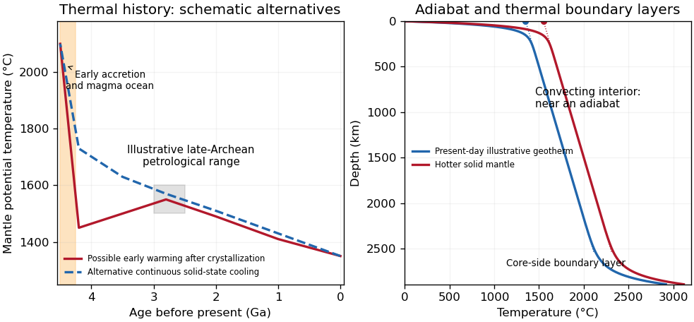
Original schematic thermal histories and mantle geotherms; curves illustrate alternatives rather than reproduce observations or fit a particular thermal model
. Details. The robust long-term picture is an energetic early Earth followed by substantial cooling and a presently mostly solid, convecting mantle. The shape of the solid-state history is less certain. Petrological reconstructions commonly place late-Archean ambient above modern values. One reconstruction infers about – at – Ga versus about today, and permits warming before that late-Archean maximum after the initial magma-ocean cooling.[ref]
Thermal history of the Earth and its petrological expression by Claude Herzberg and others. Abstract and discussion of the late-Archean temperature maximum, EPSL 292, pp. 79–88
This is a model-dependent ambient-mantle history, not proof that the accreting Earth was cooler than the Archean mantle or that every mantle reservoir followed one curve. An early molten transient, subsequent solid-state heating or cooling, and later secular cooling must be distinguished.The decisive change was from moving continents within a supposedly permanent ocean floor to moving coherent tectonic plates that include both continental and oceanic lithosphere. Several independent observations made that change testable.
Continental connections supplied the initial problem. In the early twentieth century, Alfred Wegener assembled matching continental margins, correlatable rock belts and mountain chains, shared fossil assemblages, and paleoclimate indicators into the case for continental drift. Reassembling Gondwana, for example, makes geographically separated glacial deposits and striation directions compatible with one ice-sheet system. Fits at the continental shelf edge are physically more meaningful than exact fits to modern coastlines, which have been modified by erosion and sea-level change. The evidence suggested relative movement, but did not justify the proposed forces: continents cannot readily plough independently through strong oceanic rock. A convincing mechanism and independent motion measurements were missing.
Oceanography changed the boundary conditions. Echo-sounding surveys revealed a connected spreading ridge system, axial valleys, subduction trenches and long fracture zones. Seismic refraction surveys established systematic differences between continental and oceanic crust. Thin oceanic sediment cover, high ridge heat flux and the lack of very old exposed oceanic basement made permanent, ancient ocean basins increasingly implausible. Harry Hammond Hess proposed creation of oceanic lithosphere at ridges and recycling at trenches: seafloor spreading without requiring an expanding Earth. Slow mantle convection supplied a physically plausible connection between surface transport and internal heat loss. The mechanism need not have been completely quantified before its kinematic predictions could be tested.[ref]
Developing the theory in This Dynamic Earth. Sections Ocean floor mapping, Seafloor spreading and recycling of oceanic crust
Magnetic records supplied a clock and a speedometer. Dated continental lavas established a sequence of geomagnetic reversals. Marine magnetometers then found elongated, approximately paired marine magnetic stripes on either side of ridges. The 1963 interpretation by F. J. Vine and D. H. Matthews combined repeated reversals with seafloor spreading: cooling basalt locks in remanent magnetization, and continuous motion converts a time sequence into a spatial sequence. If a polarity interval lasts and occupies width on one ridge flank, its half-spreading rate is . Matching several reversals tests the predicted sequence, rather than merely fitting a single stripe.[ref]
Magnetic Anomalies Over Oceanic Ridges by F. J. Vine and D. H. Matthews. Nature 199, pp. 947–949, magnetic striping and the spreading interpretation
Different apparent polar wander paths for different continents also became mutually consistent after continental reconstruction, favoring relative continental motion over independent magnetic-pole histories.Earthquakes identified creation, translation and consumption. Improved global seismology located shallow earthquakes along ridges and transforms, and dipping Wadati-Benioff zones beneath trenches. Their progressive focal depths identified cold, coherent slabs entering the mantle. Focal mechanisms showed extension at spreading boundaries, tangential slip at transforms and convergence at trenches. In 1965, John Tuzo Wilson's transform fault interpretation made a particularly discriminating prediction: active slip occurs between offset ridge segments, with a sense that can be opposite to that inferred by treating the entire lineament as an ordinary offset fault. The outer fracture zones are inherited traces, not continuing active plate boundaries. Agreement of focal mechanisms with the transform prediction linked magnetic and seismic evidence.
The late-1960s synthesis made these observations one quantitative theory. Relative motion of rigid tectonic plates on a sphere can be described by an Euler angular velocity vector, with . Spreading rates, transform azimuths and slip directions must fit the same rotation, and relative angular velocities must close around plate circuits. The resulting framework accounted for global boundary geometry and earthquake mechanisms without moving continents separately from the seafloor. Deep-ocean drilling beginning in 1968 subsequently confirmed that basement and overlying sediments generally become older away from ridges; this was a powerful confirmation of an already emerging synthesis, not a prerequisite discovered decades earlier.[ref]
Developing the theory in This Dynamic Earth. Sections Magnetic striping and polar reversals, Concentration of earthquakes, and discussion of the 1968 drilling programme
Thus plate tectonics succeeded through agreement between geological reconstruction, magnetic chronology, ocean-floor structure, seismology and rigid-plate kinematics. Modern satellite geodesy verifies motions directly, but belongs to the later confirmation of the theory, not its original 1960s evidence.
Coastal Kelvin-wave radiation of long Rossby waves requires a common phase convention to match the two waves. The supplied Rossby wave formula conventionally multiplies , while the coastal expression uses . Since physical fields are real, matching may use the complex-conjugate representative; in either convention the boundary forcing fixes the absolute frequency and alongshore wavenumber. Thus and .
For , the shallow-water Rossby-wave dispersion relation reduces toChoosing recovers the printed magnitude relation. Both the zonal phase velocity and zonal group velocity are approximately , so the long Rossby waves carry the coastal signal westwards into the basin.
The coastal condition alone does not guarantee a long zonal wavelength. Since , matching requires and hence the stronger consistency conditionFor example, at a coastal wavenumber with gives , which is not asymptotically small even though the meridional wavelength is long. Thus the source's proposed excitation is possible at sufficiently low frequency; it is not an automatic consequence of its meridional long-wave assumption.
At N or S the beta plane parameter isTaking a representative Pacific basin width m givesA width of – m gives roughly – years. This is propagation near latitude, not an equatorial calculation. Slow Rossby wave adjustment supplies a basin-scale delay relevant to El Niño–Southern Oscillation: changing thermocline depth can affect later sea surface temperature and coupled wind forcing. Reflection and coupling may help produce interannual memory, but this travel-time estimate alone does not establish a climate oscillation or its period.
Use Earth's rotation rate and the Coriolis parameter . At ,The Kelvin waves propagate polewards along the eastern boundary: northwards at N and southwards at S. The positive Rossby deformation radius uses ; the source's expression must be interpreted as a magnitude in the southern hemisphere.
The east-west e-folding distance is approximately km, orof longitude. With the coast at and ocean at , a northern-hemisphere snapshot can be writtenAt a positive thickness crest, the thermocline is depressed and the alongshore velocity points polewards; a negative thickness trough reverses that velocity. In the southern hemisphere replace by in the propagation and in . The envelopes of both thickness and alongshore velocity decay offshore, and the cross-shore velocity vanishes.
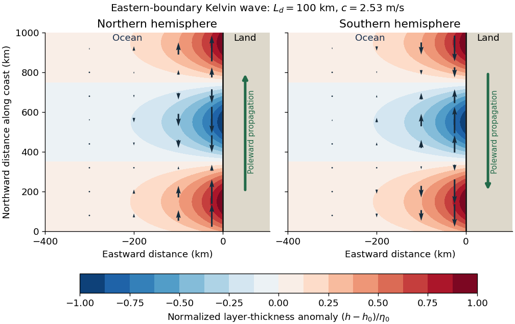
Put and . With and complex dependence , the northward momentum equation and continuity equation giveThus . Write the signed phase velocity as , so . The eastward momentum equation is the transverse geostrophic balance . HenceThe decaying sign is selected by which side of contains the ocean. For an eastern boundary the ocean occupies , so decay offshore requires . Consequently the Kelvin wave moves northwards in the northern hemisphere and southwards in the southern hemisphere, with the coast respectively on its right and left. The positive offshore decay length isThe sign of reverses the propagation direction and the sign of relative to , but not the speed or offshore decay length. The real physical fields are the real parts of the complex solution. At the equator itself this local f-plane coastal solution loses its finite trapping scale.
Use a shallow, homogeneous active upper layer of mean thickness and mass density , over a much deeper, effectively stationary layer with mass density . The Boussinesq approximation keeps the small density contrast only in buoyancy, giving reduced gravity . The hydrostatic approximation and shallow-water approximation make horizontal velocity nearly depth independent and turn the interface slope into the horizontal force .
Linearize about rest and uniform , with , neglecting products of perturbations and convective acceleration. The f-plane approximation sets the Coriolis parameter to constant . Neglect wind forcing, viscosity, entrainment and bottom drag. The two horizontal momentum equations then balance local acceleration, the Coriolis force and the pressure gradient. The signs and follow from eastward and northward coordinates.
The thickness equation is the linearized conservation of mass law: horizontal divergence decreases , while horizontal convergence increases it. Here is active-layer thickness, not total ocean depth, and rather than gives the restoring force because the motion principally displaces the thermocline.
Here , , , and , in the stated reservoir units. The exact characteristic coefficients are and , givingThe leading separation estimates give yr and yr if finite is retained, or yr if is also sent to infinity. Thus ; a ratio of ten warrants using the exact values for the requested sketch.
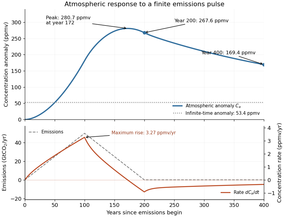
Assume initially zero anomalies in all reservoirs. The atmospheric impulse response, obtained by decomposing into the three normal modes, iswith , , and , in ppmv/GtCO. The checks and fix the instantaneous injection response and its initial decay.
The concentration is the convolution . To evaluate it transparently, define for , andsetting every when . Expressing the triangular emission history as givesHere times are in years and has the corresponding emission-ramp units. Differentiating or evaluating the convolution givesThe maximum concentration occurs earlier than the end of emissions, at approximately year , with ppmv. Initially there is a short adjustment over ; the curve then rises, turns over as emissions fall, and continues declining after year 200 as the deep ocean takes up carbon dioxide.
The total emitted mass is the area of the emission triangle, GtCO. All reservoirs eventually share one concentration, so conservation of mass gives


Define the two concentration differences and . For zero emissions and , their ordinary differential equation isWriting the positive decay rates as , their characteristic equation isConsequentlyFor , the first normal mode rapidly equalizes the fast reservoirs, giving . The slower evolution treats them as a combined capacity exchanging with , giving . ThereforeThe timescale ratio is in the joint limit. Since the conserved normal mode has , the hierarchy is .
For the linear three-reservoir carbon model, with concentrations as a column vector, the linear ordinary differential equation isA homogeneous normal mode has , where . For negative real eigenvalues the e-folding relaxation time is . The row sums vanish, so has andEqual effective concentrations generate no exchange. Summing the reservoir budgets givesThus injected carbon dioxide is conserved after emissions cease: the model redistributes it but contains no permanent removal. The zero normal mode records this conserved excess mass, rather than a long but finite decay.
To check the other normal modes are damped, set and . ThenThe similarity transformation is a symmetric negative-semidefinite matrix with a one-dimensional kernel, so the remaining two eigenvalues are strictly negative.
The constants are effective reservoir capacities: stored carbon dioxide mass anomaly per unit effective concentration anomaly, in GtCO per ppmv. Only is a literal atmospheric mole fraction; are scaled reservoir variables chosen to share its equilibrium value. The exchange coefficients are conductances, in GtCO per ppmv per year: is transfer from the atmosphere to the fast reservoir and transfer from that reservoir to the deep ocean. They are not by themselves inverse times; division by a reservoir capacity gives an inverse-time rate.
Hydrostatic balance estimates total atmospheric mass as . One ppmv of a dilute ideal gas is a mole fraction , so, with dry-air molar mass g/mol and carbon dioxide molar mass g/mol,The final factor converts kilograms to gigatonnes. This is carbon dioxide mass, not the smaller carbon mass.
Use one spectral resolution element, , and assume comparable angular resolution horizontally and vertically, so the pixel solid angle is . The question specifies only the vertical angle; without an assumption about horizontal field of view the diameter is not unique. Interpret throughput as dimensionless transmission. With primary collecting area , the power in that element iswhen is in square metres. There is no extra factor of multiplying the supplied spectral radiance.
For an integration time s, the order-of-magnitude effective noise bandwidth is Hz. The root-mean-square noise-equivalent power is then W.[ref]
NEP – Noise Equivalent Power by Thorlabs. p. 1, NEP Definition; p. 2, equations (2)–(3): minimum power and averaging time
A signal-to-noise ratio of 10 requires W, and thereforeAn ideal rectangular average of a one-sided white noise spectral density has , giving cm instead. A circular field with diameter changes the diameter by another order-unity factor. These convention choices all require an aperture substantially larger than the mm diffraction estimate, so signal collection is the stronger constraint. The estimate treats the quoted NEP as applicable to the reconstructed channel; a detailed Fourier transform spectroscopy design would also specify scan weighting, background and how interferogram noise propagates into that channel.Ignoring refraction, the line of sight is perpendicular to the radius at its tangent point. For a surface tangent, Pythagorean theorem gives the satellite-to-tangent distanceFor tangent altitude , replace by ; lower atmospheric scale heights change the estimate little. The required angular resolution isUsing the Rayleigh criterion for a circular telescope aperture, . The longest wavelength imposes the strongest condition, soThe corresponding requirement at is mm. This is a diffraction limit, without allowance for scan sampling, aberrations or instrumental field of view.
Let the two returning monochromatic fields at the chosen detector port beHere is wavenumber, rather than temporal frequency. An optical-cycle average uses and . In units absorbing the detector's field-to-power conversion,The choice of output port can reverse the cosine sign. For mutually incoherent components of the radiation spectrum, add powers rather than instantaneous fields, givingSubtracting the constant term leaves the Fourier cosine transform of the detected spectral weighting , including throughput and detector response.
The printed prefactor requires a normalization convention. In the derivation, is the amplitude of each returning field at the detector, not an entrance amplitude with input power . For a lossless balanced beam splitter and literal input power , conservation of energy instead gives , so the source formula identifies . Taking both and the printed formula literally would give at zero optical path difference, a concrete normalization contradiction.
A Michelson interferometer uses a beam splitter to divide collimated input light between a fixed mirror and a moving mirror. Returning beams recombine at the beam splitter; one output reaches a photodetector. A compensator plate can equalize the glass traversed in the two arms. Moving one mirror by changes the optical path difference by .
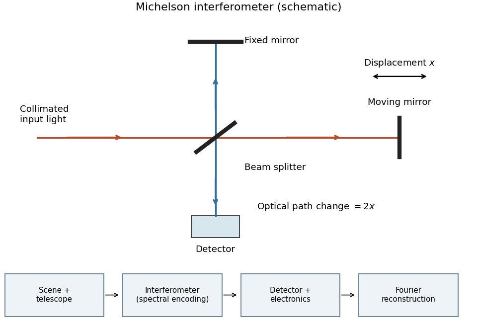
Michelson interferometer and the corresponding measurement chain
. Details. 
The usual nominal Fourier transform spectroscopy specification is , where is the maximum optical path difference measured from equal arms. It givesThis is a nominal spectral resolution element convention.[ref]
FTIR Moving Mirror Travel Distance Calculation by Thermo Fisher Scientific. optical path difference equals reciprocal resolution; mirror travel is half the optical path difference
A symmetric rectangular scan from to instead has a sinc instrumental line shape with first-zero offset . Quoting that first-zero criterion would give cm; interferogram apodization and other linewidth criteria change the numerical factor. An exact mathematical minimum requires such a criterion.In the measurement chain, the Michelson interferometer is the spectral analyzer or modulator, between the collection optics and the photodetector. It encodes the incoming radiation spectrum into an interferogram; detector electronics digitize that signal and a Fourier transform reconstructs the radiation spectrum. It does not itself turn radiant power into an electrical signal.
At the Köhler activation radius, the two coefficients satisfyConverting the atmospheric supersaturation to a fraction gives , not . Henceand the supplied curvature coefficient gives the temperatureThe coefficient and the stated radius consistently use a radius convention; replacing radius by diameter without changing the coefficient would introduce a factor-of-two error.
There are unlisted articles, also show them or only show them.