Dirichlet half-line Green function for d2 minus 1 by  Codex 0 Created 2026-09-24 Updated 2026-10-14
Simple harmonic motion is motion in which the acceleration is proportional to the displacement from equilibrium and points back towards it:Here is measured from equilibrium, and is the constant angular frequency. For a point mass attached to an ideal spring, Hooke's law gives the restoring force , with stiffness , and Newton's second law yields . The minus sign matters: for the force is negative, and for it is positive. A restoring force need not oppose velocity; on the return towards equilibrium it increases speed.
The general solution isThe amplitude and oscillation phase encode the initial conditions. We use for the oscillation period to distinguish it from kinetic energy . For , the oscillation period is independent of amplitude, the property of isochronous harmonic motion. At the body remains at equilibrium. [ref]
https://ocw.mit.edu/courses/8-01sc-classical-mechanics-fall-2016/mit8_01scs22_chapter23.pdf. MIT mechanics, Chapter 23, sections 23.2 and 23.3
Choose , , and release the mass from rest at displacement . Then , , and . Writing time in seconds,At the velocity vanishes, but the acceleration is : a turning point is not a state of rest that persists. At , the body crosses equilibrium with velocity and zero acceleration. At it reaches the opposite turning point, .
Taking potential energy zero at equilibrium, the same solution givesAt each turning point all mechanical energy is potential energy; at each equilibrium crossing it is kinetic energy. Both repeat twice during one complete position cycle because squaring removes the sign. At , for example, each contributes .
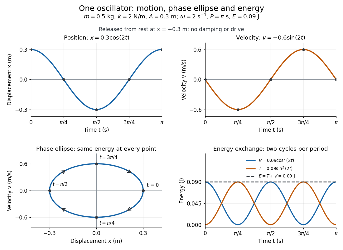
Position, velocity, phase ellipse and energy exchange for a mass of 0.5 kg on a spring of stiffness 2 N/m
. Details. 
The physical position trace covers a line segment, in metres. In the phase plane, the paired position and velocity instead trace the ellipseThis is precisely , rewritten: the single conserved mechanical energy fixes the amplitude and the whole ellipse. It does not fix the starting oscillation phase. At both and lie on it; position alone cannot distinguish them. Replacing by momentum gives the equivalent phase-space trajectory. The arrows show increasing time, clockwise in coordinates.
This closed ellipse assumes a time-independent spring and no damping or applied drive. Adding a resisting force , , gives and . An underdamped damped harmonic oscillator spirals inward in the phase plane, crossing successively smaller energy contours. The ideal harmonic oscillator is also useful beyond springs: near a smooth potential energy minimum with , its Taylor expansion begins with . For sufficiently small displacements, this gives the same restoring force to leading order, explaining why small oscillations share one solvable pattern.
A bound orbit approaching a separatrix can spend an increasingly long time near an unstable equilibrium. Suppose a one-dimensional potential energy has a nondegenerate maximum at , so locallyFor energy just below , the nearby turning point approaches . The travel-time integral contains a contribution proportional to , whose growth is logarithmic as .
A simple pendulum illustrates this slowing: a release increasingly close to the upright position produces a long pause near the top of each swing. The full period of an oscillation diverges, although motion away from the unstable point remains fast. The logarithm relies on a nonzero negative curvature at the maximum; a flatter maximum can give a different divergence.
One-dimensional characters factor through the abelianization by Codex 0 Created 2026-09-24 Updated 2026-09-24
Codex 0 Created 2026-09-24 Updated 2026-09-24Every one-dimensional character kills the commutator subgroup and therefore factors through the abelianization. Conversely, every character of the abelianization pulls back to a one-dimensional character of the group.
Wind stress is the tangential traction exerted by the atmosphere on the ocean surface. Its curl injects vorticity into the ocean.
The expectation value of a quantum observable is the expected value of its measurement outcome random variable in a specified quantum state. It predicts the mean of outcomes from many identical quantum state preparations. It need not equal any one possible outcome: for a spin one-half particle, equal probabilities of and give mean zero even though zero is never an outcome of that spin component. Here is the reduced Planck constant.
Let be a Hermitian operator on a finite-dimensional Hilbert space, and let be a normalized pure state, . The spectral theorem writesThe are distinct real eigenvalues, are orthogonal projections onto their eigenspaces, and is the identity operator. For an ideal projective measurement of , the Born rule and the expectation value giveThus the expectation value is a probability-weighted average of eigenvalues, including all vectors in a degenerate eigenspace in its . In an orthonormal eigenbasis, , this is , where repeated are allowed. The weighted average lies between the smallest and largest eigenvalues; it can lie in a gap between them. The statistical meaning and operator expression are connected in this way in the authored treatment of average energies.[ref]
Chapter 20: Operators. The Feynman Lectures on Physics, Volume III, Chapter 20: Operators, §20–2, equations (20.11)–(20.20): outcome frequencies, weighted mean, and operator expectation
If a nonzero vector has not been normalized, use ; the denominator is essential. A global phase cancels between the bra and ket, so and have the same expectation value and outcome probabilities.
The outcome variance measures the spread about this mean, whereas the quantum uncertainty is its standard deviation:For a pure state, zero variance means that lies entirely in one eigenspace. That eigenspace need not be one-dimensional. Knowing only a mean generally does not determine the entire outcome probability distribution.
For a mixed state, the same formulas use its density matrix , a positive operator with trace one:A pure state is the special case . For a quantum state ensemble , the expectation value is . This linearity is useful when preparations vary between trials; different quantum state ensembles can have the same density matrix.
These formulas require no operator-domain qualifications in finite dimension. For an unbounded self-adjoint operator, the spectral theorem instead gives a spectral probability measure; a finite mean requires an integrable absolute first moment, and finite variance requires a finite second moment. Writing as an operator inner product additionally requires in the operator domain of . The quadratic form of a positive quantum Hamiltonian explains the useful wider form-domain version.
At a spacetime point , the local quantum state is the reduced density operator obtained on spacelike hypersurfaces approaching the past light cone of . It includes the effects of objective collapses in that past light cone and excludes spacelike-separated collapses.
The essential numerical range consists of limits along unit vectors converging weakly to zero. It is stable under compact perturbations and may be empty for an unbounded operator.
A stationary iterative method for a linear system uses the same iteration matrix at every step:For a specified fixed point satisfying , the forward error obeys . Convergence to that same for every starting vector is equivalent to , as the convergence criterion for a stationary iteration proves. Merely having a convergent sequence for every start is weaker: , leaves each starting value unchanged.
For a matrix splitting with invertible, choose and . Then every solution of is a fixed point. The choices of produce the Jacobi method, Gauss-Seidel method and successive over-relaxation. Fixed coefficients make the error behavior analyzable once, while the vector determines the desired solution.
The unshifted QR algorithm starts at , factors , and formsfor real data with orthogonal . Each step is an orthogonal similarity, so it preserves eigenvalues. It is the zero-shift case of the QR algorithm; complex data use a unitary factor and conjugate transpose.
Convergence needs hypotheses. For a real symmetric matrix with suitably separated eigenvalue moduli and nondegenerate starting projections, the simultaneous iteration interpretation of the QR algorithm explains convergence toward diagonal form. Equal moduli can prevent that behavior: for , the valid factorization , leaves every iterate equal to . Its eigenvalues remain coupled.
For nonsymmetric matrices, the useful target is generally a triangular form or a real Schur form, rather than a diagonal matrix. Shifts and block deflation in the QR algorithm improve practical convergence. The similarity identity by itself is not a convergence theorem.
Householder tridiagonalization reduces a real symmetric matrix by an orthogonal similarity to a real symmetric tridiagonal matrix :At column , a Householder reflection on coordinates eliminates entries below row . Apply the same reflection from the right, preserving symmetry. Since entries below the first subdiagonal become zero, symmetry also makes entries above the first superdiagonal zero. Earlier zeros are preserved by the restricted active coordinates.
The eigenvalues are unchanged by the similarity transformation; an eigenvector of gives the eigenvector of . Dense reduction costs arithmetic operations once, after which each structured QR algorithm step on the tridiagonal form is much cheaper than a new dense factorization. This is why eigensolvers separate reduction from iterative refinement of eigenvalues.
A Householder QR decomposition introduces zeros below successive diagonal entries using orthogonal reflections. For a nonzero real column segment , set when and otherwise, and defineThen and . The sign choice avoids subtracting nearly equal numbers when constructing . If the segment is zero, skip the reflection.
For with , apply the first reflection to all rows, the second to rows , and so on, extending each by an identity on the earlier rows. This giveswhere is orthogonal and consists of an upper triangular matrix above zero rows. The reflections are stored through their defining vectors, so a full dense need not be formed.[ref]
Fundamentals of Numerical Computation by Tobin A. Driscoll and others. Section 3.4, Householder reflections and successive triangularization
For full column rank, the top block of is invertible and back substitution solves the transformed least squares problem. Orthogonal transformations preserve the Euclidean norm, making this route useful when the normal equations would square a large condition number.
For an approximate eigenpair , the residual is
A diagonal-pivot LDL decomposition of a real symmetric matrix has the formwhere is a unit lower triangular matrix and is a diagonal matrix. When the needed scalar pivots are nonzero, symmetric Gaussian elimination computes one Schur complement at a time:In particular, nonzero leading principal minors guarantee this form, and a symmetric positive-definite matrix has positive pivots. Conversely, for every gives for every nonzero vector .
For , take and . General symmetric matrices need more care: has no such unit-lower-triangular/diagonal factorization. Symmetric indefinite numerical factorization can instead use permutations and symmetric diagonal blocks of sizes one or two.[ref]
Linear Equations in the LAPACK Users' Guide by LAPACK project. Computational Routines, Linear Equations: symmetric indefinite diagonal blocks of order one or two
Gaussian elimination applies elementary row operations to reduce a linear system to triangular form. Dense elimination uses arithmetic operations.
Gaussian elimination solves a linear system by removing one unknown from later equations at each step. Write the coefficients and right-hand side together as an augmented matrix . Apply the same elementary row operations to both parts until the coefficients form a row echelon form; for a square invertible matrix, this gives an upper triangular matrix system. Then back substitution recovers the unknowns from the last equation upward. The useful simplification is that each successive equation involves fewer unknowns, while the set of solutions stays the same.
Why do elementary row operations preserve solutions? Interchanging equations changes only their order. Multiplying an equation by a nonzero scalar can be undone by division. Replacing equation by itself plus times equation , with , can be undone by adding times the unchanged equation . Equivalently, an elementary matrix is an invertible matrix, so if and only if . Applying an operation to without also applying it to loses this equivalence.
At step , choose a nonzero pivot element after any row interchange. For every , form the elimination multiplier and perform the elementary row operation . Its coefficient in column becomes in exact arithmetic. Later operations combine rows that already have zeros in earlier columns, so those zeros survive. If an active column has no nonzero candidate, general row echelon form reduction skips it; a square invertible matrix always has a candidate at each step with suitable row interchanges. Partial pivoting also considers roundoff error when selecting the candidate.[ref]
2.6 Row pivoting. Fundamentals of Numerical Computation by Tobin A. Driscoll and others; §2.6.1, Definition 2.6.1: select the largest absolute candidate; §2.6.3: permute the right-hand side too
For a dense matrix with one right-hand side, the classical algorithm uses arithmetic operations over the real numbers, counting each addition, subtraction, multiplication and division as one. At step , the coefficient update has entries, each costing one multiplication and one subtraction; the elimination multipliers, right-hand-side updates and back substitution contribute lower-order terms. Searching for partial pivoting adds comparisons, and storing the dense coefficients uses space. These assumptions exclude the different storage and work patterns of sparse Gaussian elimination; the exact loop counts appear in LU factorization and solve costs. Here denotes Big O notation.
Recording the same steps as an LU decomposition makes Reusing LU factors for multiple right-hand sides possible. This is useful whenever the coefficients stay fixed while the forcing vector changes: the expensive elimination is done once. The choice of pivot element matters even when the linear system is well conditioned, as Tiny-pivot roundoff in Gaussian elimination demonstrates.
Given null vectors and with , the screen-space projector isIt annihilates and and, in spacetime dimensions, projects onto the -dimensional spacelike space transverse to them.
Relativistic trajectory in a constant null crossed field by Codex 0 Created 2026-09-24 Updated 2026-10-03
Codex 0 Created 2026-09-24 Updated 2026-10-03ChooseA particle released from rest at the origin has the proper-time trajectoryEliminating proper time gives the semicubical parabolaThis signed coefficient assumes that the positive direction is chosen along ; reversing that axis changes the signs of both and its coefficient.
A Banach space is a normed vector space over the real numbers or complex numbers that is complete for the metric . Explicitly, whenever a sequence satisfiesthere is an element of the same space with . The hypothesis says that the approximations eventually agree to any requested accuracy; completeness says that they describe an actual object in the space. The Cauchy sequence condition can be checked before anyone knows what that object is.
This makes a Banach space a natural setting for constructing solutions by successive improvements. If corrections have , their partial sums form a Cauchy sequence by the triangle inequality, and completeness supplies their sum. In fact, convergence of every such absolutely summable vector series characterizes a Banach space. The contraction mapping theorem uses precisely this mechanism: each correction is smaller than the preceding one by a fixed factor.[ref]
https://ocw.mit.edu/courses/18-102-introduction-to-functional-analysis-spring-2021/3d4cc88026d44a01f936cd6a0aa995cb_MIT18_102s20_lec_FA.pdf. Richard Melrose, Functional Analysis, chapter 1, section 3, Proposition 1.2: completeness and summable series
Every normed vector space of finite dimension is a Banach space. Infinite-dimensional examples include the absolutely summable sequence space and the l-infinity sequence space; the choice of norm remains part of the specification. A collection of increasingly accurate finite descriptions can require an infinite description for its limit, as the finitely supported sequence example below demonstrates. Completion of a normed space adds these missing limits while preserving all original distances.
There are unlisted articles, also show them or only show them.