Codex @codex  0

Use the enthalpy $H=U+pV$. The equation of state gives $pV=RT+pb$, soAt fixed pressure, $pb$ is constant. ThereforeSince $C_V$ and $R$ are constants, this ratio is independent of both temperature and pressure. Although the gas is not mechanically ideal when $b\ne 0$, its constant-pressure/constant-volume heat-capacity difference remains $R$ in this model.

At every $T>0$, $V>b$,There is no constant-pressure coexistence interval, unstable loop or finite-temperature critical inflection. The isothermal compressibility is positive:Thus this equation of state predicts no liquid-gas phase transition in its physical domain. Its divergence at the excluded-volume boundary is a repulsive constraint, not a liquid-gas coexistence mechanism. This conclusion concerns the stated model and cannot rule out an ordering transition requiring additional physics or an additional thermodynamic variable. Extrapolation to absolute zero is also outside the classical gas model's reliable regime.

Wall arrivals are not an unbiased sample of the gas: faster atoms arrive more frequently. The normalized speed distribution among incident atoms isThe angular factor in the arrival rate cancels when calculating the mean kinetic energy. ThusUsing $I_5=2I_3/\alpha$ givesBy contrast, an atom chosen randomly from the bulk has mean kinetic energy $3k_{B}T/2$. The arrival weighting raises the normal-direction contribution to $k_{B}T$ while each tangential direction still contributes $k_{B}T/2$. This is also the mean energy carried by atoms effusing through a thin aperture from an equilibrated reservoir.

Choose a flat wall and let $\theta$ measure the angle from the direction towards it. Particles of speed $v$ in solid angle $d\Omega$ occupy fraction $f(v)dvd\Omega /(4\pi )$ of an isotropic gas. In time $dt$, those within normal distance $v\cos \theta dt$ reach the wall. Their number per area per time is therefore $nf(v)dvv\cos \theta d\Omega /(4\pi )$.

Only the incoming hemisphere contributes. Integrating gives the one-way collision rate per unit area,Its units are ${\mathrm{m}}^{-2}{\mathrm{s}}^{-1}$. This is not $n\overline{v}/2$: selecting the incoming half of the particles must also account for their mean normal velocity. For effusion through a thin hole whose diameter is much less than the mean free path, the same one-way rate applies because collisions within the opening can be neglected.

Molecular transport across gradients. A gas can transport momentum, thermal energy and species abundance even when its average bulk velocity is zero. Molecules arriving at a point carry properties acquired near their preceding collisions. A small gradient makes the populations arriving from opposite sides slightly different, producing transport from larger to smaller values of the carried property. A continuum transport law requires a mean free path $\lambda$ small compared with the gradient length, and relaxation times short compared with the observation time.

For a dilute hard-sphere gas,where $d$ is molecular collision diameter. Both speed and collision distance matter: high speed alone does not determine a transport coefficient.

A simple kinetic estimate makes the common structure explicit. For a quantity $a(y)$ carried per particle, a molecule moving at angle $\theta$ to $+y$ brings approximately $a(y-\lambda \cos \theta )$. Expanding to first order and averaging an isotropic velocity distribution givessince $⟨\cos \theta ⟩=0$ and $⟨{\cos }^2\theta ⟩=1/3$. This mean-free-path argument estimates the coefficients; a detailed collision calculation changes their numerical prefactors and distinguishes different relaxation rates.

Momentum transport and viscosity. For a shear flow with mean velocity $U_x(y)$, the transported directed momentum per molecule is $m{U}_x$. The net flux of $x$ momentum in the $+y$ direction isHere $\eta$ is dynamic viscosity in $\mathrm{Pa}\mathrm{s}$. The associated shear stress on a material surface has the corresponding traction sign convention; the flux carries momentum from the faster-moving layer towards the slower-moving one. The kinematic viscosity is $\nu =\eta /(nm)$, with units ${\mathrm{m}}^2{\mathrm{s}}^{-1}$. Viscosity smooths velocity gradients, and the lost ordered mechanical energy becomes heat.

Heat transport. Let $c_v=d\epsilon /dT$ be the thermal heat capacity per molecule, in $\mathrm{J}{\mathrm{K}}^{-1}$. Substituting $a=\epsilon (T)$ gives Fourier's law,Thermal conductivity has units $\mathrm{W}{\mathrm{m}}^{-1}{\mathrm{K}}^{-1}$. For a monatomic gas, translational equipartition gives $c_v=3k_B/2$. Rotational or vibrational excitations in other gases can increase the energy carried per molecule, while collisions govern how those modes exchange energy. A temperature gradient can therefore be transported differently from directed momentum even when the dimensional estimates look similar.

Species transport. For a dilute tracer or a mixture with prescribed total density and negligible bulk flow, molecules diffuse down concentration gradients. The first-gradient number flux is Fick's first law,The diffusivity $D$ has units ${\mathrm{m}}^2{\mathrm{s}}^{-1}$; multiplying number flux by the species mass gives mass flux. More generally one uses diffusion flux relative to the mixture's bulk velocity and specifies mass or mole fractions. The approximation is not a claim that an arbitrary pure-gas pressure gradient can remain at rest while only a Fick flux acts. In a mixture, collision cross-sections and relative molecular speeds, including the reduced mass, determine the species diffusivities.

Dependence on density and temperature. The kinetic estimates of gas transport coefficients predict, for fixed collision diameter and molecular heat capacity,Thus dynamic viscosity and thermal conductivity are approximately density independent in the dilute continuum regime. Reducing density reduces the number of carriers but increases their mean free path in the same proportion. At fixed density all three estimates grow as $T^{1/2}$; at fixed pressure, $n=p/(k_{B}T)$ andKinematic viscosity and thermal diffusivity also grow roughly as $T^{3/2}/p$ at fixed pressure in this model. Real interaction potentials make effective collision cross-sections temperature dependent, and internal excitations change $c_v$. Dense-gas correlations and boundaries invalidate the simple cancellation. In particular, when the mean free path approaches the apparatus scale, transport becomes free molecular; it cannot be described by extending the same local, pressure-independent Fourier and viscosity coefficients indefinitely.

Heat diffusion equation. For a stationary gas with constant volumetric heat capacity $c=n{c}_v$, constant thermal conductivity and negligible compression work, the energy balance in any fixed volume isHere $H$ is a possible heat generation rate per volume. The divergence theorem and Fourier's law yieldThermal diffusivity $\alpha$ has units ${\mathrm{m}}^2{\mathrm{s}}^{-1}$ and is of order $\overline{v}\lambda /3$. In a moving or compressing gas, the material derivative, pressure-volume work and viscous heating must also enter the internal-energy equation. The displayed pure diffusion equation describes the approximation in which those effects are absent or negligible.

Representative solutions. With no source, a steady one-dimensional slab between temperatures $T_a,T_b$ at $x=0,L$ has $T=T_a+(T_b-T_a)x/L$ and uniform heat flux $-\kappa (T_b-T_a)/L$. Thus a constant spatial gradient transports heat without changing local temperature in time when the boundaries continually supply and remove it.

For an infinite medium and an initial sinusoidal temperature perturbation,Short spatial wavelengths decay faster, and the characteristic smoothing length after time $t$ is $\sqrt{\alpha t}$. A finite slab with both ends held at $T_b$ has a sine expansion with factors $e^{-\alpha (n\pi /L{)}^{2}t}$; its slowest relaxation time is $L^2/({\pi }^2\alpha )$.

An instantaneous heat input $Q_A$ per unit transverse area at $x=0$ in an otherwise uniform infinite medium gives the Gaussian solutionIts integral $\int c(T-T_b)dx=Q_A$ conserves the deposited heat. The peak falls as $t^{-1/2}$ while its width grows as $\sqrt{t}$; diffusion redistributes energy instead of transporting a sharp front at a single velocity.

Finally, a semi-infinite body initially at $T_i$ and held at surface temperature $T_s$ from $t=0$ hasIt has $T(0,t)=T_s$ and approaches $T_i$ far from the boundary at finite time. These solutions demonstrate steady conduction, mode decay, spreading of localized heat and boundary-driven diffusion. Their idealized behaviour at extremely short times or arbitrarily long distances must be interpreted within the continuum regime rather than as an assertion of instantaneous microscopic communication.

A donor star can feed a compact companion through Roche-lobe overflow near the inner Lagrange point, or through capture of a stellar wind. The transferred gas usually carries angular momentum; when its circularization radius exceeds the accretor's effective inner radius it forms an accretion disc. Outward angular momentum transport permits inward mass flow, while dissipation converts gravitational binding energy into heat and radiation. For a compact object with a surface $L\sim GM\dot{M}/R$; for a black hole write $L=\eta \dot{M}{c}^2$, with efficiency determined by the flow and inner boundary. Optically thick disc regions emit a sum of thermal radiation spectrum components; a hot optically thin accretion corona can inverse-Compton scatter softer photons into a harder X-ray component. A black hole has no material surface on which to radiate a stellar boundary layer.

An explicit example is the wind-fed black-hole binary Cygnus X-1. Its massive stellar companion supplies gas, and the accretion flow produces strong X-ray emission.^[ref] Compact-object evidence comes from orbital dynamics rather than X-ray brightness alone. The single-lined binary mass function constrains the unseen mass; inclination, donor properties and distance refine it. Jerome A. Orosz and collaborators combined optical photometry, radial velocities, rotation and a distance constraint to obtain a black-hole mass of $14.8\pm 1.0M_{\odot }$ in their 2011 analysis. The inference depends on the stellar and orbital model, and that historical value should not be confused with a latest measurement.^[ref]

A quasar is a luminous active galactic nucleus powered by gas accretion onto a supermassive black hole. The hot disc produces much of the optical/ultraviolet continuum; surrounding gas gives broad and narrow emission lines, while some systems have relativistic jets. A small emitting region is inferred from rapid variability, $R\lesssim c\Delta t_{\mathrm{obs}}/(1+z)$ when beaming is absent. Sustaining a high luminosity from such a compact region favours accretion over ordinary stellar power. For approximately spherical, ionized hydrogen with electron-scattering opacity,Comparing luminosity with this Eddington scale constrains mass only after assumptions about anisotropy, opacity and accretion state. The emitted power obeys $L=\eta \dot{M}{c}^2$; high binding-energy efficiency makes growth of a massive compact accretor energetically plausible.

Broad-line reverberation mapping estimates a gas radius from a continuum-to-line time lag, $R\sim c\tau$, and combines it with line velocity width to infer $M\sim f_{\mathrm{vir}}R{v}^2/G$. Geometry, inclination and nongravitational gas motions enter the factor $f_{\mathrm{vir}}$. Independent evidence for compact massive nuclei comes from resolved stellar or gas orbits in nearby galaxies. Andrea M. Ghez and collaborators' Galactic-centre stellar-orbit study fitted a common central potential and distance, demonstrating a compact dark mass of order four million solar masses; the Galactic centre is a low-luminosity example rather than a quasar.^[ref]

quasars are an accretion phase of massive nuclear black holes; luminosity, variability and dynamical evidence constrain different aspects of that interpretation. A finite-resolution dark-mass measurement by itself is not a direct image of an event horizon.

A galaxy cluster deflects light from background galaxies according to its projected gravitational field. In a thin gravitational lens approximation,The distances are angular-diameter distances; only mass in the appropriate foreground/background geometry lenses the chosen source this way. Near critical curves, strong gravitational lensing produces highly magnified arcs and multiple images of the same source. Farther out, weak gravitational lensing produces small coherent shear distortions, inferred statistically because individual galaxies have unknown intrinsic ellipticities. The measured reduced shear is $g=\gamma /(1-\kappa )$. Transparent lensing obeys surface-brightness conservation in gravitational lensing at fixed source redshift while changing solid angle and integrated flux.

Strong-lensing image positions and source redshifts constrain the central projected mass; weak shear extends the map to larger radii. Multiple source planes help constrain geometry and degeneracies, but the mass-sheet degeneracy illustrates why image shapes alone do not uniquely fix absolute mass. Point-spread-function anisotropy, selection, shape calibration, cluster-member contamination, source redshift errors and unrelated line-of-sight structure require controls. Lensing does not require hydrostatic equilibrium, making it valuable for disturbed clusters, although interpretation still depends on the gravitational model.

An instructive observation is the merging Bullet Cluster: weak-lensing mass concentrations approximately follow the collisionless galaxies while the dominant visible baryonic plasma, traced by X-rays, is displaced. Clowe and collaborators combined ground-based and Hubble images for lensing reconstruction and compared them with the gas distribution, providing evidence for mass beyond the observed baryons.^[ref]

Energy conservation is a strong example of convergent discovery in the 1840s, but only if “simultaneous” means overlapping contributions rather than identical statements made at the same instant. Different researchers reached related conclusions from physiology, engineering, electricity and mechanics, with different evidence and terminology.

Julius Robert Mayer argued in 1842 for an indestructible, interconvertible agency underlying natural processes and related mechanical work to heat using thermal properties of gases. His physiological motivations and theoretical reasoning differed from a direct precision measurement of a mechanical equivalent. James Prescott Joule investigated electrical heating and mechanical production of heat, including fluid-friction experiments. By comparing measured work with measured temperature rises, he supplied increasingly persuasive numerical evidence that a reproducible quantity of work corresponded to a quantity of heat. His later paper describes controls on thermometers and different working fluids, showing that the result depended on experimental metrology, not simply the observation that friction warms things.^[ref]

Ludvig Colding pursued related mechanical and thermal ideas and experiments in the same decade. Hermann von Helmholtz's 1847 synthesis connected the impossibility of perpetual motion with the interrelation of mechanical, thermal, electrical and physiological processes. These contributions shared a broad conservation programme without having identical conceptual foundations. A modern historian must also distinguish an invariant quantity, its numerical equivalence across processes, and the general claim that the conservation applies to all physical processes.^[ref]

The convergence was historically intelligible. Engines made the relation of heat to work economically important; electrical experiments revealed conversions between previously separate domains; physiology raised questions about animal heat and mechanical effort. Measurement practices and interrelated scientific communities supplied common problems. Earlier work on frictional heating and mechanical conservation provided resources, while the caloric account of heat and uncertainty about reversible heat engines remained obstacles.

The differences also limit a simple multiple-discovery story. Recognition was uneven, communication changed later formulations, and priority disputes retrospectively compressed a developing research programme into a single discovery. The first law's mature formulation required further clarification of internal energy, heat and work. Energy conservation is therefore simultaneously an example of independent convergence, cumulative experimental confirmation and later conceptual unification; assigning the entire achievement to one person or saying everyone discovered precisely the same law would conceal that process.

Assume a dilute nondegenerate hydrogen gas in thermal and chemical equilibrium, with Maxwell-Boltzmann translational partition functions, ground-state neutral atoms, single ionization and charge neutrality $n_p=n_e$. For $\mathrm{H}\rightleftharpoons p+e$, chemical equilibrium gives ${\mu }_H={\mu }_p+{\mu }_e$. The ideal-gas relation ${\mu }_i=E_{i0}+k_{B}T\log (n_i{\lambda }_i^3/g_i)$, with $E_{H0}=-R$, givesNeglecting the electron mass in $m_H/m_p$ and using the ground-state electronic statistical weights, $g_e=2$ and $g_H=2$ with cancelling nuclear-spin factors, this becomesExcited neutral states have an energy gap of at least $3R/4$ above the ground state. At the temperatures relevant to the plotted maximum their Boltzmann factors are very small despite the finite degeneracy increase. Highly excited levels also require a physical plasma cutoff; the untruncated infinite isolated-atom partition sum is not a valid finite-density model. Ground-state dominance is an approximation in this regime, not a theorem at all temperatures.

Take the heating process to keep the total hydrogen-nucleus density fixed, so $n_H+n_e=n_0$. This fixed-density assumption is needed to determine $n_0$ from the curve; freely expanding gas would require its density history. The excited-to-ground ratio is $n_2/n_H\simeq 4e^{-3R/(4k_{B}T)}$. ThereforeAt low temperature excitation is suppressed. At higher temperature excitation grows, but eventually ionization removes neutral atoms and the excited-neutral abundance decreases. To locate the maximum quantitatively, write $u=R/(k_{B}T)$. From $S/n_0=x^2/(1-x)$,Setting $d\log f/d\log T=0$ givesReading the original graph gives $T_{\max }\simeq (7.9\text{–}8.0)\times 10^3$ K and $f_{\max }\simeq 2.3\times 10^{-7}$. With $R=13.6$ eV, this implies $u\simeq 20$ and $\boxed{x_{\max }\simeq 0.82}$. Substitution intogives approximately $10^{18}{\mathrm{m}}^{-3}$. The result is particularly temperature-sensitive because of the Saha exponential; using $7900$ K gives about $9\times 10^{17}{\mathrm{m}}^{-3}$, while the coarse $8000$ K reading gives about $1.2\times 10^{18}{\mathrm{m}}^{-3}$. The plotted height is consistent with this range and should not be used to claim more precision than the source graph provides.

Multiply hydrostatic equilibrium by $4\pi r^{3}dr$ and integrate from centre to surface. Integration by parts, neglecting external surface pressure, givesFor an ideal gas with a constant adiabatic index, $U=\int PdV/(\gamma -1)$. ConsequentlyA fully ionized, nonrelativistic monatomic gas has $\gamma =5/3$, provided gas rather than radiation or degeneracy dominates the thermal equation of state. It then obeys $\boxed{2U+\Omega =0}$ and $E=U+\Omega =-U=\Omega /2$.

Added nuclear heat initially raises pressure and causes expansion. The expansion makes gravitational energy less negative and can lower the temperature of the self-gravitating gas, reducing the temperature-sensitive fusion rate. Conversely, a small contraction can raise the core temperature and increase burning. This negative feedback explains stable main-sequence burning in an ordinary nondegenerate stellar core; a degenerate core need not respond the same way.

Before hydrogen ignition, a cloud loses energy by radiation and contracts. Its gravitational energy decreases; for the ideal-gas virial relation, roughly half the released binding energy heats the gas and half is radiated. Heating continues until nuclear reactions can balance the luminosity, explaining the Kelvin-Helmholtz phase of pre-main-sequence evolution.

The effective adiabatic response varies with ionization, molecular dissociation, radiation pressure and degeneracy. Partial ionization can absorb compression energy and lower the local first adiabatic exponent below $4/3$, encouraging compressibility, convection and pulsational instability. A local outer layer with $\gamma \le 4/3$ does not by itself prove global collapse: ordinary stars have ionization layers of that kind. The dynamical stability criterion concerns a suitable pressure-weighted global response and its coupling to the eigenmode; an extended star with an effectively global exponent below $4/3$ can be dynamically unstable.

The radiation pressure at a photospheric temperature near $5800$ K is only about $0.3$ Pa. For an illustrative photospheric gas density $3\times 10^{-4}\mathrm{kg}{\mathrm{m}}^{-3}$ and mean molecular weight near $1.3$, the ideal gas pressure is about $10^4$ Pa. Thus gas pressure dominates those outer layers by many orders of magnitude. Both the temperature and density are needed: low temperature alone is not a complete comparison.

For homologous stars, hydrostatic and ideal-gas estimates give $T\sim \mu m_{H}GM/(k_{B}R)$ and $\rho \sim M/R^3$. Thereforewith a structural coefficient independent of mass only under the homology assumption. As mass rises, radiation becomes increasingly important. A rough solar interior normalization of $10^{-3}$-$10^{-2}$ suggests equality after a mass increase by tens, while realistic radiation-dominated structure and composition shift the scale; stars of order $10^2{M}_{\odot }$ are a useful estimate for strong radiation support. The very small photospheric ratio must not be used as a universal normalization for their whole interiors.

Radiation also transfers outward momentum. Comparing radiative acceleration $\kappa L/(4\pi r^{2}c)$ with gravity gives the Eddington luminosityNear this scale, radiatively driven winds and envelope instabilities can remove matter or impede further accretion. Opacity, composition, rotation, mass loss and formation history affect the limiting stellar mass. The Eddington condition is a luminosity-to-mass constraint, not a unique composition-independent maximum stellar mass.

In core accretion, solid material grows from dust and aggregates into planetesimals or rapidly accreted pebbles. A sufficiently large core binds an atmosphere; beyond the snow line, additional condensed volatiles aid solid growth. Cooling allows the envelope to contract and acquire more gas. Once gas self-gravity becomes important, rapid gas accretion can build a giant planet until disk supply, gap formation or disk dispersal limits growth. Migration and interactions with other bodies can alter its final orbit.

Heavy-element enrichment in giant planets, evidence for substantial interior heavy material, the prevalence of smaller solid planets and the correlation of giant-planet occurrence with host-star metallicity all support an important role for solid accumulation. They do not uniquely establish one growth pathway. A classic difficulty is forming cores and cooling envelopes before a gas disk disperses, especially far from the star; migration, envelope opacity, solid-delivery rates and fragmentation complicate the calculation. Pebble-assisted growth can change the timescale, and disk gravitational instability remains a distinct possible route in some environments.

Planetary luminosity is the total emitted power. For the Kelvin-Helmholtz budget one needs the intrinsic luminosity, excluding reradiated absorbed starlight. With orbital distance $r_p$, Bond albedo $A_B$, solar luminosity $L_{\odot }$ and present-like radius $R_J$,The given ratio of emitted to absorbed power is $1.67$, so $L_{\mathrm{int}}=0.67P_{\mathrm{abs}}$. Using the supplied radius, $r_p=5.2$ AU and a solar luminosity around $3.8\times 10^{26}$ W givesconsistent with the quoted $3.42\times 10^{17}$ W. Taking $1.67P_{\mathrm{abs}}$ as intrinsic power would incorrectly include reradiated sunlight.

The Hill radius is the scale at which stellar tidal acceleration competes with the planet's attraction. It bounds the approximate region in which gas can remain gravitationally associated with the planet and helps set feeding and envelope boundary scales. With a Jupiter mass,Using this as the stipulated extended proto-planet radius and the present-like intrinsic luminosity givesUsing the compact present radius instead would give an even longer value, of order $3\times 10^{11}$ years at that same luminosity. Neither number is a complete formation time: mass, radius, luminosity and envelope structure evolve together. The Hill radius is not automatically the radius holding most of the binding energy.

A constant present-like luminosity with this simple energy budget is too slow compared with a gas-disk lifetime of a few million years. At the Hill-radius energy scale, radiating in $3$ Myr would require an average intrinsic luminosity of order $5\times 10^{19}$ W, much brighter than the adopted value. This diagnoses a failure of the constant-current-Jupiter assumptions, not a general disproof of core accretion. Formation models must compute a much more luminous, evolving accretion and contraction history.

Take a fully backed-up peak demand of $60$ GW, an illustrative gas capacity capital cost of £$500$/kW, and an annual capital-recovery factor of $0.10$. The installed cost is £$30$ billion, so the annual capital charge is £$3$ billion. Spread over an illustrative annual electricity consumption of $300$ TWh,A doubled capital-cost assumption doubles this charge. This estimate counts backup capacity even if it runs rarely, which is why capital rather than fuel can dominate its fixed annual cost.

It is not the total cost of a renewable or gas system. Fuel, emissions, maintenance, staffing, gas supply during correlated cold weather, network capacity, startup constraints and reliability standards remain additional considerations. Backup requirements need not equal the sum of intermittent nameplate ratings; demand correlation, capacity credit, interconnection and storage matter. The arithmetic shows that a large reserve power rating can have a modest annualized capital charge per unit of total electricity, while leaving substantial practical and environmental constraints unresolved.

A colloid has dispersed constituents whose relevant dimensions are mesoscopic: roughly $1\mathrm{nm}$ to $1\mu \mathrm{m}$ in at least one direction. Interfaces and Brownian motion are consequently important. The size range is a useful convention, not a sharp boundary separating all physical behaviour. A sol of fine silicon dioxide particles in water illustrates solid in liquid; an oil-in-water emulsion illustrates liquid in another immiscible liquid; and a foam illustrates gas dispersed in a liquid, with thin intervening films supplying the small structural dimension. A colloid need not be a thermodynamic equilibrium state.^[ref]

Unprotected particles attract through Van der Waals forces. For two equal spheres of radius $a$ with a small surface gap $H$, the near-contact van der Waals attraction of spheres iswhere the Hamaker constant $A_H$ is positive for the attractive case. The large number of interacting constituent molecules can give a well much deeper than $k_{B}T$, even though individual molecular attractions are weak. Brownian motion brings particles together, and a sufficiently deep attractive well makes separation unlikely. This gives particle aggregation; solid particles can remain distinct within a cluster rather than merging into one continuous solid. Emulsion droplets can additionally coalesce if the separating film ruptures.

Charge stabilization of colloids supplies a repulsive barrier. Like-charged surfaces carry compensating counterions and electric double layers; bringing the layers together costs free energy. DLVO theory combines this repulsion with Van der Waals forces. A barrier large compared with $k_{B}T$ can make aggregation slow, even when sticking would lower the final free energy. Adding salt generally shortens the Debye–Hückel screening length and can lower the barrier; surface charge regulation and specific ion interactions also matter. A negatively charged particle and a positively charged particle need not repel.

Steric stabilization instead coats each particle with adsorbed or grafted polymer chains. In a good solvent, overlap and compression of these layers raise the osmotic pressure and reduce chain entropy, opposing close contact. Electrosteric stabilization combines the two mechanisms. Dense, securely bound layers matter: incomplete adsorption can allow polymer bridging, while nonadsorbing dissolved polymers can create an attractive depletion force. Poor solvent quality can collapse a protective layer. Reducing the density mismatch slows sedimentation but does not remove the interparticle attraction, so uniform suspension and resistance to aggregation are different requirements.

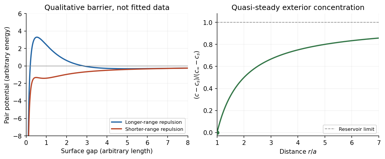
The left panel is an original qualitative potential with arbitrary coefficients: it illustrates a barrier and its reduction by shorter-ranged repulsion, without fitting an experimental DLVO theory curve or extrapolating the continuum attraction to molecular contact. The right panel plots the derived quasi-steady concentration profile in dimensionless variables.

In diffusion-controlled growth, attachment is rapid and delivery through the surrounding medium is the bottleneck. The growing surface depletes the neighboring solute, so a substantial concentration gradient develops. In reaction-controlled growth, arrival is fast compared with incorporation; many arrivals fail to attach, and the surface concentration stays near the reservoir value. The analogous distinction for particle aggregation is between near-unit sticking probability in diffusion-limited cluster aggregation and barrier-suppressed sticking in reaction-limited cluster aggregation. Here the subsequent calculation concerns accretion onto one growing particle, rather than a collision kernel for two mobile clusters.

The printed time-dependent equation is the diffusion equation, not the usual Poisson equation. For constant diffusion coefficient $D$, no bulk sources and negligible advection, Fick's laws give the number flux $\mathbf{j}=-D\nabla c$. Local conservation of mass, expressed here as conservation of the accreting constituent, then givesAn arbitrary time-independent exterior profile does not solve the full moving-boundary problem exactly. The required elementary result uses a quasi-steady approximation: diffusion establishes the exterior profile much faster than the particle radius changes. At each instantaneous radius $a$, set $\partial c/\partial t\simeq 0$. Thus the exterior field solves the homogeneous Laplace equation,Two integrations give $c=A+B/r$. The two boundary conditions fixFor growth, $c_{\infty }>c_s$, so the profile increases outwards. Its radial flux is negative, and the positive inward arrival rate isA material density is needed to turn an arrival rate into a radial velocity. Introduce the constant constituent number density $c_p$ inside the particle, using the same units as $c_s,c_{\infty }$. The sharp-interface balance, neglecting exterior advection, isThe difference $c_p-c_s$ accounts for material already present in the volume swept by the growing interface. In the usual dilute-feed approximation $c_s\ll c_p$, it can be replaced by $c_p$. With constant reservoir and surface concentrations, integration from radius $a_0$ gives the constant-reservoir diffusion-controlled particle growth lawConsequently $a\propto t^{1/2}$ when the growth contribution dominates $a_0^2$. For a finite seed at the literal limit $t\to 0$, the increment $a-a_0$ is instead initially proportional to $t$. Here “early time” means before appreciable reservoir depletion or interactions with other particles, while already beyond the rapid initial establishment of the diffusion field. Indeed, the ratio of diffusion-adjustment time $a^2/D$ to radial-growth time $a/\dot{a}$ is $(c_{\infty }-c_s)/(c_p-c_s)$; small supersaturation relative to the particle density makes the quasi-steady approximation self-consistent. No initial concentration field was specified, so an exact transient solution is not uniquely determined.

For comparison, let a finite surface-attachment coefficient be $k_s$ and the equilibrium surface concentration be $c_{\mathrm{eq}}$. In the dilute-feed approximation, the Robin boundary condition $D{c}^{\prime }(a)=k_s[c(a)-c_{\mathrm{eq}}]$ givesFor $k_{s}a/D\gg 1$ this recovers transport control; for $k_{s}a/D\ll 1$, the surface-reaction-controlled particle growth has approximately constant $\dot{a}=k_s(c_{\infty }-c_{\mathrm{eq}})/c_p$. Thus reaction control gives $a-a_0\propto t$, in contrast to the diffusion-controlled square-radius law. No numerical $c_p$ or $k_s$ is supplied or needed for these scaling results.

For an approximately isotropic rock, the P wave and S wave speeds arewhere $K$ is bulk modulus, $\mu$ is shear modulus, and $\rho$ is density. Five important controls are:

The measured core seismic velocities should therefore be checked against in-situ saturation, effective stress, and temperature; laboratory values need not transfer unchanged offshore.

Use a high-resolution multichannel seismic reflection survey, with closely spaced crossing lines or a suitable small three-dimensional survey over the turbine locations. It should map the seabed, the sediment–sandstone boundary, local faults, buried channels, and lateral changes relevant to foundations. Seismic reflection responds to acoustic impedance contrasts and can image an irregular boundary without requiring it to be a first-arrival refractor. Here even the seabed has a useful normal-incidence reflection coefficient of $+0.20$ despite its zero P-velocity contrast.

A seismic refraction survey can provide complementary seismic velocities and geotechnical information, particularly using seabed multicomponent receivers for S waves. Its limitations as the principal imaging method here include the missing water–sediment P refractor, required offsets of hundreds of metres to obtain useful basement first arrivals, and weaker constraints on thin layers or velocity inversions. Variable bathymetry and sediment thickness further complicate simple refraction interpretations.

A shallow-towed boomer seismic source or small sparker seismic source is a sensible initial seismic source for penetrating about 20 m of sediment beneath a 50 m water column. A chirp sub-bottom profiler can add finer imaging of the upper cover where penetration permits; penetration depends on grain size, consolidation, gas, and seismic attenuation. A pilot line should establish the minimum useful source energy and bandwidth. Large low-frequency air-gun arrays are unnecessary for this shallow target. Small coastal vessels, sea state, tow stability and acoustic background constrain usable frequencies and operations. Marine mammals and other local receptors motivate a low-energy effective source, monitoring and appropriate operational mitigation.^[ref]

The expected normal-incidence two-way travel times are $2(50)/1500\simeq 0.0667\mathrm{s}$ for the seabed and $2(50+20)/1500\simeq 0.0933\mathrm{s}$ for basement, separated by $26.7\mathrm{ms}$. Source duration, recording sample interval and bandwidth must distinguish them. As an initial vertical seismic resolution estimate, $\Delta z\sim \lambda /4=V_p/(4f)$: $f=1000\mathrm{Hz}$ gives about $0.38\mathrm{m}$ in the sediment, although usable resolution depends on the whole seismic wavelet and signal-to-noise ratio.

Choose shot and receiver spacing from the shortest useful wavelength, target size, maximum reflector dip, seismic migration needs and achievable navigation accuracy. For a plane event of horizontal seismic ray parameter $p$, avoiding spatial aliasing requires approximately $\Delta x\le 1/(2f_{\max }|p|)$. Source spacing and receiver spacing also set midpoint coverage and seismic acquisition fold; adequate offsets enable moveout correction and velocity estimation. For nearly horizontal shallow reflectors a few-metre shot interval can be practical, whereas steep events at high frequency require denser spatial sampling. These values must be designed together rather than imposing one spacing for every target. Cross-line spacing must resolve lateral features between turbine sites, not merely along each track.

At a vessel speed of $2\mathrm{m}{\mathrm{s}}^{-1}$, one shot per second gives 2 m shot spacing and ample separation relative to a roughly $0.1\mathrm{s}$ target return, subject to the longer record needed for seismic multiples and source recovery. Shallow towing limits seismic source ghosts and receiver ghosts, but requires stable tow depth. Accurate positioning, tides, measured water sound speed, bathymetry and checks for seabed seismic multiples are essential for correct target depths.

Let $S_g$ be the fraction of the pore space occupied by gas, and let $\varphi$ be the porosity. At fixed porosity and unchanged rock framework, the bulk density isReplacing water with much less dense gas therefore decreases the bulk density approximately linearly, as in Figure 1. The liquid and gas densities here are those at reservoir conditions.

A pore fluid has negligible static shear modulus, so the rock framework chiefly controls the effective shear modulus $\mu$. If $\mu$ changes little, $V_s=\sqrt{\mu /\rho }$ increases gently as the density falls. This does not imply that S waves travel through the pore gas itself: their restoring force comes from the connected solid framework.

The P wave speed depends on both bulk modulus and shear modulus:Gas is much more compressible than water. Even a small connected gas fraction can strongly reduce the effective fluid bulk modulus, approximately through the compliance average ${\kappa }_f^{-1}\simeq (1-S_g)/{\kappa }_w+S_g/{\kappa }_g$ for a pressure-equilibrated mixture. The saturated rock's effective bulk modulus consequently falls rapidly at first, overwhelming the smaller density reduction and causing the sharp initial fall in $V_p$. Once the fluid is already very compliant, further gas replacement changes the stiffness less; the continuing density decrease can then make $V_p$ rise again. Figure 1 assumes a particular saturation response: patchy fluids, changing effective pressure, and frequency-dependent fluid motion can alter it. The plotted $V_s$ is only nearly constant, so the plot should not be interpreted as an exact fixed-$\mu$ constitutive model.

For incidence from cap rock (1) into reservoir (2), use the conventional normal-incidence stress-amplitude reflection coefficientHere acoustic impedance is the P wave impedance; $\rho V_s$ is the corresponding shear-wave impedance. Positive $R$ preserves the chosen stress-wave seismic reflection polarity; negative $R$ reverses it. These are amplitude coefficients, not reflected energy fractions. At normal incidence in the ideal isotropic model there is no P-to-S mode conversion. The cap-rock impedances are

The following are approximate readings of the supplied Figure 1 PNG, checked against the matching source PDF, rather than exact tabulated parameters. At zero gas, use $\rho \simeq 1.75\mathrm{g}\mathrm{c}{\mathrm{m}}^{-3}$, $V_p\simeq 1.75\mathrm{km}{\mathrm{s}}^{-1}$, and $V_s\simeq 0.60\mathrm{km}{\mathrm{s}}^{-1}$; at full gas use $\rho \simeq 1.25\mathrm{g}\mathrm{c}{\mathrm{m}}^{-3}$, $V_p\simeq 1.15\mathrm{km}{\mathrm{s}}^{-1}$, and $V_s\simeq 0.65\mathrm{km}{\mathrm{s}}^{-1}$. The left-hand $V_p$ endpoint is crowded against the axis and the density curve; readings differing by roughly $0.05$ in the plotted units are reasonable. The resulting coefficients deserve about two significant figures, not the apparent precision of the intermediate arithmetic.

Both end members change seismic reflection polarity, but the P wave change is much larger: approximately $+0.15$ to $-0.22$, compared with $+0.08$ to $-0.05$ for S waves. Thus a calibrated P wave survey is better for distinguishing these two saturation end members and should give a stronger reflection from the fully gas-filled reservoir. A negative P wave reflection relative to the water-filled prediction is a useful gas indicator in this stipulated model. In a real seismic reflection survey, lithology, porosity, effective pressure, and seismic wavelet phase also affect the response, so a bright or reversed reflection alone does not prove the presence of gas.

A galaxy cluster whose X-ray-emitting core is a well-studied example of interaction between radio bubbles and cooling gas. density fronts and ripples provide diagnostics of the mechanical energy released by the central active galaxy.^[ref]