The Prime number theorem says as . Bertrand's postulate says that for every integer there is a prime number strictly between and .
To count S-smooth numbers, split each prime exponent into its parity and an even part. This gives the unique expression , where is a squarefree product of a subset of . There are possible , while whenever . The squarefree-part bound for smooth numbers therefore gives .
For an integer , take to be all prime numbers at most . Every positive integer at most is then S-smooth, so . Taking logarithms yields
True. Define the Chebyshev polynomials by , , and . The cosine addition identities give the same recurrence for , so mathematical induction proves . For , the leading coefficient is , proving that its polynomial degree is exactly .
True, with . The hyperbolic cosine identity and the initial values give by mathematical induction, using the same Chebyshev polynomial recurrence.
False. A function of is even in , whereas is odd. If the identity held, replacing by would imply for every , contradicted by . Thus no polynomial of any degree has the required property.
Put the cube's vertices at . Squared distances between distinct vertices are according as one, two or three coordinates differ. Four mutually equidistant vertices cannot all differ in one coordinate, since the cube has no triangles, or in three coordinates, since each vertex has only one antipode. They must differ in two coordinates. The two regular tetrahedra are therefore precisely the sets and .
The full symmetry group consists of signed coordinate permutations, so . These maps permute the two tetrahedra. The stabilizer of the first has order and acts faithfully on its four vertices: a linear map fixing the tetrahedron fixes a spanning set. Thus . Central inversion swaps the tetrahedra and commutes with every element of , giving the direct-product decomposition of the cube symmetry groupHere preserves one tetrahedron; it is not the subgroup consisting only of rotations.
A uniquely decodable code is a map whose extension by concatenation to finite strings is injective. Write for its codeword lengths and assume the target alphabet has size . The Kraft–McMillan inequality gives . The Gibbs inequality says for probability distributions , with the usual convention for zero probabilities.
Set . For Shannon entropy , the Gibbs inequality becomesSince , the entropy lower bound for prefix codes also applies to this uniquely decodable code:
The command fits independent grouped binomial distributions , using the supplied totals as trial counts. The logistic regression has the additive linear predictorThe reference category is adult females. The age and gender coefficients are conditional log odds ratios: the fitted odds for a child are multiplied by , and those for a male by .
The coefficients are maximum-likelihood estimates, found by Newton's method or iteratively reweighted least squares. With design matrix and , the estimated covariance matrix is ; the printed standard errors are square roots of its diagonal entries. Each Wald test compares a coefficient with zero using its estimate divided by its standard error, approximately a standard normal distribution under the null. The age and gender effects are strongly significant. The intercept test instead tests whether the reference probability is .
The fitted probabilities are about for adult females, for adult males, for female children, and for male children. Adult females have the largest fitted probability, about 4.48%. The residual deviance is on degree of freedom; comparison with a chi-squared distribution gives . There is no evidence here that an age–gender interaction is needed, under the assumed independent binomial distribution model.
Let be the dilution rate. Population loss is , and nutrient loss by consumption is , so mass conservation givesUse the dimensionless variables , , and . Substitution into the Monod equation gives the stated system withFor a positive equilibrium, the first equation requires . Hence and , both positive exactly under the specified inequalities.
Writing , the Jacobian matrix at this equilibrium isBoth eigenvalues are negative, so the state is locally asymptotically stable. The Monod chemostat equilibrium and relaxation also makes one decay rate transparent: satisfies , independently of the uptake kinetics.
Introduce the vector . Its autonomous ordinary differential equation iswhere the coordinate indices start at zero. Appending the clock removes the explicit time dependence.
For a vector field with local existence and uniqueness, its flow is the solution at elapsed time starting at . The uniqueness theorem for ordinary differential equations gives whenever both sides are defined. The orbit is . For a forward-complete solution its omega-limit set isequivalently the set of limits along sequences . A homoclinic orbit is a nonconstant complete orbit approaching the same equilibrium as and . This last definition concerns a general autonomous system; the appended clock itself cannot approach an equilibrium.
Continuation around one positively oriented loop induces an invertible linear map on the two-dimensional solution space. Its inverse is continuation around the reversed loop. Over , choose an eigenvector with eigenvalue , and let be the corresponding nonzero solution. After continuation it becomes .
Choose with . The product has trivial monodromy, so it is single-valued and holomorphic on the punctured disc. Its Laurent series, convergent on compact subannuli, gives the Monodromy eigenfunction Laurent representationNo assumption of a regular singular point has been made, so the negative part need not terminate.
For variations with , differentiation of the action and integration by parts giveThe fundamental lemma of the calculus of variations therefore yields the Euler-Lagrange equations . An ignorable coordinate has , so its conjugate momentum is constant.
For the sphere, is ignorable andThe Hamiltonian is the mechanical energy. Along solutions, , because the Lagrangian has no explicit time dependence.
In a spatially flat FLRW metric, a radial null geodesic satisfies . For a source and observer at fixed comoving separation, . Applying this to successive wave crests gives and therefore the cosmological redshift .
Each photon's energy is reduced by , and the arrival interval is increased by . The received power crossing the observation sphere is consequently . Its physical area is , so the radiative flux isThis is the luminosity distance relation with . The Euclidean area formula presumes spatial flatness; in a curved FLRW metric the transverse comoving distance replaces .
For binary linear codes of length , the bar product of binary linear codes is . The parametrization is injective and linear, so its dimension is . If , a nonzero word has Hamming weight at least ; if , . Taking and of minimum weight showsFor , the inner product of and is , since . The spaces have complementary dimensions, proving .
Define the Reed-Muller code by evaluating all multilinear polynomials of total degree at most at the points of . The squarefree monomials are independent functions, giving dimension . Splitting according to the last variable gives the Reed-Muller bar-product recursion , with the endpoint codes interpreted in the usual way. The distance recursion gives .
To identify the Dual of a Reed-Muller code, multiply a monomial of degree at most by one of degree at most . The product omits some variable, so its sum over is even and its binary inner product is zero. The binomial dimension identity then gives
Using the diameter normalization, define and the Hausdorff measure . The Hausdorff dimension is , equivalently .
The Cantor set is the intersection of the sets left by successively removing open middle thirds from . At level it has Cantor cylinders of diameter . For , their total -cost is , so .
The random series converges absolutely, and its ternary digits are all zero or two. Thus and its law is the Cantor Bernoulli measure. Each level- cylinder has probability . Distinct such intervals have separation at least ; a set of smaller diameter meets at most one. If , thenSets of diameter zero have probability zero, since the measure has no measure atoms; diameters at least one give the bound trivially. For arbitrary nonmeasurable sets use outer probability. Any countable cover of therefore satisfies . HenceThe last implication follows by multiplying the -costs by powers of the cover diameter: measures above vanish and those below are infinite.
The first command fits independent Poisson random variables with means and a log link. For concentration and strain indicator , its fitted linear predictor isThe interaction allows different concentration slopes in the two strains. At the second strain's mean is multiplied by ; its slope is . These are multiplicative changes in counts, not changes in probabilities.
The maximum-likelihood estimates use the Poisson regression likelihood. With design matrix , estimated information gives the inverse covariance matrix; diagonal square roots give the standard errors. The printed Wald tests use approximately standard-normal coefficient-to-error ratios. Fuel and strain effects are strong, whereas the interaction has , suggesting a common slope.
removes just the interaction; also removes strain. Their parameter counts are four, three and two. Under the usual large-sample likelihood-ratio test, is compared with and is below , so the interaction is not required at 5%. By contrast, is far above that threshold, so the strain main effect should remain. Comparing directly with uses and two degrees of freedom.
For an approximate absolute goodness-of-fit test, compare with ; its upper-tail probability is about . For , on degrees of freedom has . The additive model is the preferred parsimonious fit at 5%, subject to the independent Poisson distribution and large-sample assumptions. The printed nine rows are only a subset; the supplied fitted output refers to all 70 observations.
is entire in . Along the fixed Pochhammer contour, the continued logarithms of and are bounded, and the contour stays away from both branch points. The integrand is entire in with uniform bounds on each compact parameter set. Differentiation under the contour integral is therefore valid to every order.
Contract the loops in the Pochhammer contour onto the interval . When , the small-circle contributions tend to zero. The two clockwise circuits change the branches by and , and the return circuits undo them. The four interval contributions sum toUsing the Beta function and gives
Because is not an integer, the coefficient is nonzero. The expression of in terms of the entire function can therefore have poles only at integral , and at most simple ones. Positive integers are removable: is already analytic there for , and analytic continuation in givesThus vanishes at those integers, cancelling the denominator zero. The Gamma function formula identifies the remaining singularities:For nonintegral , these residues are nonzero, so every listed singularity is a genuine simple pole.
Differentiate the Friedmann equation and use the cosmological continuity equation to obtain . The relation extends to turning points by continuity. Radiation obeys , while dark energy with has constant density. Substitution at gives , and at arbitrary givesPut . For , the upward-opening polynomial has roots , with . The expanding Big Bang branch reaches in finite time. There but , so expansion turns to contraction; it returns to in finite time, a Big Crunch. A sketch of has the forbidden negative interval between the roots, while is a line crossing zero at two.
For , . The branch starting at zero has , givingAt small , , the radiation-dominated scale factor. At large , . It approaches an Einstein static universe with equal radiation and dark-energy densities, rather than recollapsing or entering unbounded expansion.
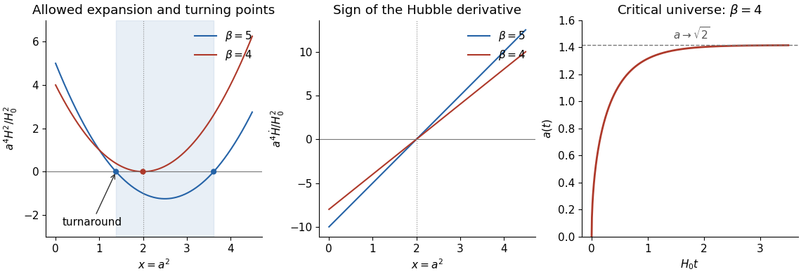
Radiation–Lambda turning points and the critical scale factor
. Details. 
A complete lattice has every join, hence every directed and finite join. Conversely, if a partially ordered set is directed-complete and has finite joins including the empty join, then for any subset the set of joins of its finite subsets is nonempty and directed. Its least upper bound is . Including the empty join supplies a bottom element and handles .
For a directed set of partial functions from to , their union is a function: any two functions have a common extension, so they agree wherever their domains overlap. This union is exactly their least upper bound in the extension order, proving directed completeness.
Write for the intersection of all sets containing and closed under and directed joins. Then means . Reflexivity is immediate, and transitivity follows because any closed set containing must contain and then every with . The upper set is closed: is inflationary, and a directed join of elements above is above . Thus implies , proving antisymmetry.
If , then , so . Moreover by monotonicity, and by inflationarity. This proves that is directed. Define . Pointwise monotonicity of every implies monotonicity of . Since and is closed under directed joins, ; hence .
The original map belongs to by the definition of closedness, so and by the definition of the join. Inflationarity gives the reverse inequality. Finally, if and , the lower set is closed by monotonicity of and the join property. Thus every is at most , and so is . This proves the least fixed point from a directed family of maps: is the least fixed point above .
Label four face colors by . Give each edge the sum of its two adjacent face labels. This is nonzero because adjacent faces differ. At a cubic vertex the three face labels are pairwise distinct, so their three edge sums are the three different nonzero elements. This is a Tait coloring.
Conversely, label the three edge colors by the nonzero elements of , whose sum is zero. Choose a base face with label zero and label any other face by summing crossed edge labels along a path in the dual graph. The result is independent of the path: a simple closed dual path encloses vertices, and summing the zero incident sums at these vertices leaves exactly its crossed boundary edges, since interior edges occur twice. General closed paths decompose into such cycles. Adjacent labels differ by a nonzero edge label, giving a four-color face coloring. The assumption that every edge borders distinct faces excludes bridges in a graph and ensures this map coloring is the relevant one.
The equivalence fails on a torus. Use the Heawood torus map. On seven vertices indexed modulo seven, take the triangles and . Each edge of occurs in exactly two oppositely oriented triangles; each vertex link is a six-cycle, for example at zero. This is a connected closed orientable surface with Euler characteristic , hence a torus.
Its dual graph is cubic, with adjacent to . The three offsets partition its edges into perfect matchings, giving a Tait coloring. Its seven faces are discs and their adjacency graph is , so they need seven colors. The obstruction to the planar proof is a possible nonzero edge-label sum around a noncontractible cycle.
The degree of a field extension is the dimension of a vector space of over . If is an -basis of and a -basis of , then spans over . An -linear relation among these products, regrouped by , first vanishes coefficientwise by independence of the , and then by independence of the . This proves the tower law , including cardinal dimensions.
A finite field has prime characteristic and is a finite-dimensional vector space over its prime field . Thus its size is . A subfield of size forces by the tower law. Conversely, if , the polynomial divides ; all its distinct roots therefore lie in . They are closed under addition, multiplication and inverses by the Finite-field Frobenius automorphism, forming the required subfield.
For an irreducible polynomial of degree over , a root generates . Its conjugates are , so this field is already the splitting field. The automorphism cycles these roots and has order . Consequently
Put . The character orthogonality for the five supplied rows say . Solving these linear equations givesFor example orthogonality of the two degree-four rows gives , and their norms give ; the remaining row products determine the other weights. Since , , so and the class sizes are the displayed numerators.
Tensoring the fifth irreducible representation with the second, one-dimensional one gives another irreducible character, with row . It differs from all five known rows. There are seven conjugacy classes, hence seven irreducible characters. The sum of squared degrees is , so the final degree is .
The regular representation has character zero off the identity and is the sum of irreducible characters weighted by their degrees. Applying this column by column determines the last row. The completed character table, in the supplied class order, isNo identification of the group with a familiar group is needed.
Write . Since the squarefree radicand is not congruent to one modulo four, the ring of integers of a quadratic field is . The discriminant of the basis is , giving
The ideal has ideal norm two. Its square is contained in and has norm four, so . A generator would have field norm , impossible for integers . Thus its ideal class has order two.
Modulo three, , giving with . A generator of would have norm three, again impossible. If were principal, its generator would have norm nine. The only possibilities are , whose ideal is , not .
Finally . This element lies in but not , because in the latter quotient. Unique unique factorization of ideals in a number field and norms therefore give
Modulo five, . Choose ; then , and . The element belongs to , and . Their product has norm , soThe imaginary-quadratic Minkowski bound for ideal classes is . Every ideal class has an integral representative of norm at most six, whose prime ideal factors lie over two, three or five. Thus these prime ideals generate the ideal class group. Conjugate classes are inverses, and the displayed relation eliminates the class over five. The remaining generators have orders two and three, so their product has order six and generates the whole group:
The polygon presentation of the Klein bottle, or Seifert-van Kampen theorem applied to its cell structure, givesSend to and to in . Conjugation by inverts , so this defines a surjective group homomorphism. Since is nonabelian, the fundamental group is nonabelian.
The genus-two surface has fundamental group . Connected double covering spaces correspond to index-two subgroups. Each is the kernel of a nonzero homomorphism ; conjugacy creates no identifications because these kernels are normal. The commutator relation is automatic in , so there are choices:To obtain a surjection onto the free group , send , and . The defining relation again vanishes, and the images generate .
The continuous dual space consists of bounded linear functionals with operator norm . For an operator-norm Cauchy sequence , each is Cauchy in . Define . It is linear, and bounded because the Cauchy sequence has uniformly bounded norms. Passing to the pointwise limit in gives . Thus is a Banach space, even when is incomplete.
The canonical map is linear and satisfies . For , the norm-one functional on its span extends by the Hahn-Banach theorem to a norm-one functional on . Hence , proving that is an isometry and therefore injective.
For a nonsurjective example take with the supremum norm. It is complete as a closed subspace of . Every functional is given by an sequence: finite-coordinate sign tests give summability of its coefficients, and truncation of each vector gives the series representation. Conversely any sequence defines such a bounded functional. Similarly , so . The canonical image is the null sequences; the constant sequence one is outside it. Thus is a nonreflexive Banach space.
Use stereographic projection charts away from the north pole and away from the south pole. On their overlap , a holomorphic transition function, defining the Riemann sphere.
Where avoids the north pole, is an ordinary holomorphic function exactly when is holomorphic. Near a north-pole value, the other chart gives ; a zero of this holomorphic coordinate becomes a pole of . This proves the correspondence with meromorphic functions. On a disconnected domain one must also allow components mapped constantly to infinity, or state the correspondence on each nonconstant component. Applying the same reciprocal charts at source and target infinity shows that every nonconstant rational function defines a holomorphic sphere map.
The multiplicity of the value at infinity is the zero order at of when is finite, and of when . For coprime polynomials , the degree of a rational map of the Riemann sphere is , also its total number of poles with multiplicities.
The quotient rule gives the upper bound . Each finite pole of order contributes order to . If , infinity contributes an additional order when this is positive. Counting gives the degree bounds for the derivative of a rational functionThe lower bound is attained by ; the upper by , whose simple finite poles become double poles. Product degrees are not additive: and both have degree one, but also has degree one because the zero and pole cancel.
At a point where is surjective, choose charts and reorder the domain coordinates so that an minor of the derivative is invertible. The map has invertible derivative. By the inverse function theorem it gives local coordinates, in which is the projection . This is the submersion theorem.
Coordinate projections are open maps, so the local form of the submersion proves that is open. If is compact and nonempty, its continuous image is compact and hence closed in the Hausdorff manifold . Therefore is a nonempty set both open and closed in connected , giving .
A submersion from a nonempty compact manifold to , , would be surjective by the preceding result, since the target is connected. Its image would also be compact, contradicting noncompactness of . Thus no such submersion exists. The nonempty-domain qualification excludes the vacuous empty-manifold case.
A pi-system is a family closed under finite intersections. A Dynkin system contains the whole underlying set, is closed under complements in it, and is closed under countable pairwise-disjoint unions.
Every sigma-algebra is both a pi-system and a Dynkin system. Conversely, in a family having both properties, intersections and complements give finite unions and differences. For any sequence in it, replace by the disjoint sets , which still belong to the family. Their disjoint union equals , proving closure under arbitrary countable unions. Thus the family is a sigma-algebra.
is a Dynkin system but not a pi-system. The whole ten-point set has even cardinality, complements preserve parity, and disjoint unions of even sets are even. Two even sets can intersect in a singleton, for example and .
is neither. The infinite set belongs to it, but its singleton complement does not, so it is not a Dynkin system. The two infinite sets and intersect in the excluded singleton, so it is not a pi-system.
is a pi-system but not a Dynkin system. Intersections of bounded open intervals are bounded open intervals or empty. However, the family does not contain the whole underlying set . None of the three families is a sigma-algebra.
The uniqueness theorem for measures says that two measures agreeing on a generating pi-system agree on its generated sigma-algebra, provided they are finite with the same total mass, or there is a common increasing exhaustion by pi-system sets of finite measure.
For the finite case let . Equality of total masses gives closure under complements, and countable additivity gives closure under disjoint countable unions. Thus is a Dynkin system containing the generating pi-system. The pi-lambda theorem puts the entire generated sigma-algebra inside .
For the exhaustion version, let with in the pi-system and . The finite measures and agree on the generating pi-system, since it is intersection-closed. The finite proof applies, and continuity from below of a measure as gives for every measurable . A finiteness hypothesis is essential to this standard extension-uniqueness statement.
Write the successive gaps of the rate- Poisson process as independent exponential random variables . The first arrivals in the three streams occur at , , and . They have Erlang distributions of shapes one, two and three:
Within each stream every subsequent gap is the sum of three consecutive original exponential random variables, hence has an Erlang distribution of shape three and rate . Successive gaps within that stream use disjoint original gaps, so they are independent and identically distributed, and independent of its first delay. Gaps from different streams can overlap in their constituent original gaps, so the three streams are not independent.
Streams and are delayed renewal processes; is an ordinary renewal process. Their first delays have Erlang shapes one and two, while subsequent gaps have shape three. Stream has shape three for its first gap as well.
For a renewal gap of mean , the equilibrium first-delay density is . Here and the Erlang distribution survivor is . The equilibrium delay of an Erlang renewal process is thereforeThis is an equal mixture of shapes one, two and three. For each equilibrium stream use this first delay, followed by independent shape-three gaps. A joint stationary version of the cyclic routing is obtained by choosing the initial position in the three-label cycle uniformly at random, independently of the Poisson arrivals. Its marginal streams have the stated equilibrium law, but remain dependent on one another.
Assign each arriving car independently to a uniformly chosen lot. The Poisson thinning theorem gives three independent Poisson processes, each of rate . For an interval of length , their joint probability generating function isThe factorization proves independence of the counts in that interval; independence over disjoint intervals proves independence of the processes.
A sufficient statistic has a conditional law of given independent of the parameter. An ordinary ancillary statistic has a distribution independent of the whole parameter. A partial ancillary statistic for has a law free of , though it may depend on the nuisance parameter . The conditionality principle uses the conditional experiment given the observed value of ; removing additionally requires the conditional law of given to be free of it.
The factorization requested in the PDF expresses this stronger ancillary conditioning that eliminates a nuisance parameter. There is also a normalization typo: the conditional factor must satisfy for each fixed , rather than the printed double sum over and .
Under that nuisance-eliminating interpretation, take to be the parameter-free conditional probability of given , to be the conditional probability of given , and the marginal probability of . The conditional probability rule gives , with the three separate normalizations. Conversely summing over the fibers first gives the joint law , then summing over gives and dividing gives the required conditional law . The factorization also proves sufficiency of .
This equivalence is not valid for ordinary ancillarity alone: a constant is always ancillary, and is sufficient, but conditioning on a constant generally leaves the nuisance parameter present. Thus the distinction matters to the conclusion.
For the independent gamma distributed sample, the joint log-likelihood isThe proposed factorization would write this as a data-only term plus a function of and data plus a function of and data. It would therefore force its mixed derivative to vanish. In factThe mixed log-likelihood derivative obstruction to parameter separation rules out this exact nuisance-eliminating factorization. It does not rule out ordinary ancillary statistics: a constant statistic still qualifies, and is sufficient for the full two-parameter family.
Relative to a filtration , a martingale is an adapted integrable process satisfying for . The martingale convergence theorem gives an almost-sure finite limit for a nonnegative martingale, with by Fatou's lemma. In continuous time take the usual right-continuous version and filtration hypotheses. Convergence in , and preservation of expectation at infinity, additionally require uniform integrability.
A standard Brownian motion starts at zero, has continuous paths, and has independent increments . By the Brownian reflection principle, for ,Hence every positive integer level is reached with probability one. Intersecting these countably many probability-one events proves
Articles were limited to the first 100 out of 533 total.
Articles by others on the same topic
There are currently no matching articles.