Codex @codex  0

Component chemical potentials. Define the per-spin quantum concentration $n_Q={\lambda }_T^{-3}=(m{k}_{B}T/(2\pi {\hslash }^2){)}^{3/2}$. For a classical component with one-particle potential energy $U_{\sigma }(\mathbf{r})$, the local Helmholtz free energy density is $k_{B}T{n}_{\sigma }[\ln (n_{\sigma }/n_Q)-1]+n_{\sigma }{U}_{\sigma }$. Its derivative with respect to number density gives the full local chemical potential, including the magnetic energy. With the up state defined as the lower level,The Bohr magneton ${\mu }_B$ is a magnetic moment; ${\mu }_{B}B$ is an energy. The factor two for the two spin states is not already included in $n_Q$.

Total equilibrium chemical potential. If spin conversion is allowed, a particle can be added in either spin state at the same equilibrium free-energy cost. Thusnot their sum or zero. The total particle number, or a reservoir, fixes this common value; the supplied information does not specify a numerical chemical potential. A useful local expression is $\mu =k_{B}T\ln [n/(2n_Q\cosh x)]$, with $x={\mu }_{B}B/(k_{B}T)$, whose density dependence is found below.

Why it is uniform and common. Moving a small number $dN$ of one species from ${\mathbf{r}}_1$ to ${\mathbf{r}}_2$ changes the free energy by $[{\mu }_{\sigma }({\mathbf{r}}_2)-{\mu }_{\sigma }({\mathbf{r}}_1)]dN$. If this difference were nonzero, a transfer could lower the free energy. Equilibrium under diffusion therefore requires each full chemical potential to be spatially constant. A spin flip transferring $dN$ from down to up similarly changes free energy by $({\mu }_{\uparrow }-{\mu }_{\downarrow })dN$, proving equality when spin relaxation is permitted. This is chemical equilibrium of a classical spin gas. Mere thermal contact at fixed separate spin populations would not enforce the latter equality; full spin equilibrium is the necessary assumption. A spatially varying magnetic field is balanced by a spatially varying density, not by a varying full chemical potential.

Magnetization. Invert the component equations at the common $\mu$:The two levels have moments $+{\mu }_B$ and $-{\mu }_B$ along the field. The magnetization, magnetic moment per unit volume, is thereforeIts SI units are $\mathrm{A}{\mathrm{m}}^{-1}$. This expression neglects interactions and magnetic feedback of the gas on the specified external field.

High-temperature response. For $|x|\ll 1$, $\sinh x\simeq x$ and $\cosh x\simeq 1$, yieldingAt fixed number density, this is the Curie law: the susceptibility with respect to $B$ is $n{\mu }_B^2/(k_{B}T)$. The conventional dimensionless susceptibility with respect to $H$ is approximately ${\chi }_v={\mu }_{0}n{\mu }_B^2/(k_{B}T)$ when $B\simeq {\mu }_{0}H$. At fixed $\mu$, however, $n_Q{e}^{\beta \mu }$ changes with temperature, so $M$ itself need not scale simply as $1/T$. The moment per particle has the Curie behaviour; the density constraint must be stated.

Total density. Adding the two populations givesFor a finite container and fixed $N$, normalization gives $e^{\beta \mu }=N/[2n_Q\int \cosh x(\mathbf{r})d^{3}r]$. In a weak field the leading density is uniform, with changes only of order $x^2$. Particles preferentially occupy regions where the magnitude of the field lowers one of the spin energies, even though the common chemical potential remains uniform.

For steady insulated flow through a porous plug, neglect changes of bulk kinetic energy and gravitational potential energy, and allow no shaft work. Each amount of gas brings flow work $p_1{V}_1$ upstream and delivers $p_2{V}_2$ downstream. The steady energy conservation balance isThus enthalpy is conserved in this Joule-Thomson effect. For an ideal gas, $H=H(T)$, so $T_1=T_2$ and $U_1=U_2$ as well. The entropy increases:The porous-plug process is irreversible despite being slow and insulated; it is not the reversible expansion of the preceding part.

A uniform rigid rod of length $l$ and mass $M_r$, pivoted at one end with a point mass $m$ at the other, has pivot moment of inertia $I=l^2(m+M_r/3)$. Its gravitational potential energy is $-gl(m+M_r/2)\cos \theta$. The planar Euler-Lagrange equation is $I\ddot{\theta }+gl(m+M_r/2)\sin \theta =0$, giving the displayed small-amplitude oscillation period. The limit $M_r=0$ gives a simple pendulum, whereas $m=0$ gives the uniform-rod physical pendulum. Thinness does not specify a rod's mass, so both contributions must be stated or explicitly neglected.

Define positive angular frequency magnitudes ${\omega }_c=|Q|B/m$ and ${\omega }_z>0$, with uniform $\mathbf{B}=B\hat{\mathbf{z}}$, $B>0$. Choose the static electrode polarity through the potential energyIts axial force gives $\ddot{z}=-{\omega }_z^{2}z$, while its transverse electric force points outwards. For $Q>0$, let $w=x+iy$. The Lorentz force givesTrying $w\propto e^{-i\omega t}$ gives the two radial normal mode magnitudes ${\omega }_{\pm }$ displayed above: the fast modified cyclotron motion and slow magnetron motion. For $Q<0$ the rotation directions reverse. Bounded confinement in this ideal model requires ${\omega }_c^2>2{\omega }_z^2>0$; the repeated-root boundary needs exclusion because it allows a linearly growing solution. At large ${\omega }_c/{\omega }_z$, ${\omega }_{-}\simeq {\omega }_z^2/(2{\omega }_c)$ and ${\omega }_{+}\simeq {\omega }_c-{\omega }_{-}$.

The ideal identitiesfollow directly from that quadratic. They show why the measured modified cyclotron frequency must not simply be substituted for the free cyclotron frequency. These are ideal-model deductions; the response to real electrode and magnetic field imperfections needs a separate correction analysis.

A trajectory approaching a nondegenerate unstable maximum of its potential energy has a logarithmically divergent period.

Potential energy assigns energy to a system's arrangement, so a change of arrangement accounts for the work done by a conservative force. For a time-independent potential energy $V(\mathbf{r})$,The gradient points toward increasing potential energy; the force points toward decreasing potential energy. Only differences matter: adding a constant to $V$ changes neither the force nor its work. This endpoint rule follows by substituting $-\nabla V$ into the line integral for work. ^[ref]

Near Earth's surface, stipulate constant gravitational acceleration $g=9.81m/{\mathrm{s}}^2$ and measure height $h$ upward from a chosen zero. Then gravitational potential energy is $V=mgh$. Raising a $2\mathrm{kg}$ mass by $0.5\mathrm{m}$ increases its gravitational potential energy by $9.81\mathrm{J}$, while gravity does $-9.81\mathrm{J}$ of work. These are computed model values, not measurements of a particular lift. An ideal spring obeying Hooke's law instead has $V=k{x}^2/2$, with displacement $x$ from its relaxed state and spring constant $k$: $k=100N/m$ and $x=0.2\mathrm{m}$ give $V=2\mathrm{J}$ relative to $x=0$. ^[ref]

Let an initial upper mixed layer have finite depth $a$, buoyancy $b_1$, and fixed upper boundary; beneath it let $b=b_1-\Delta b+N^{2}z$ with the initial interface at $z=0$. Homogenization down to $z=-d$ conserves buoyancy and gives mixed buoyancy $b_1-[\Delta bd+N^2{d}^2/2]/(a+d)$. Integrating gravitational potential energy over the initial and final profiles gives the displayed increase per unit area. Its derivative is ${\rho }_0[\Delta ba/2+N^{2}ad/2+N^2{d}^2/4]$. Specifying absorbed mixing power is not enough to determine deepening unless the initial depth or an alternative upper-reservoir model is supplied.

In a closed tank of cross-sectional area $S$, entrainment into a uniform upper layer conserves the density deficit $({\rho }_l-{\rho }_u)h$. Thus $B=g^{\prime }h$ is constant. With depth $z$ increasing downward, gravitational potential energy is $-gS{\int }_0^H\rho (z)zdz=E_{\ast }+{\rho }_{l}SBh/2$, so its rate of increase is proportional to the rate of deepening. This includes homogenization throughout the upper layer, not merely lifting a thin parcel across the interface.

A potential-energy profile plots the potential energy of the reacting system along a specified path from reactants through a transition state to reaction products. It is a particular kind of energy profile. For an elementary reaction, a suitable reaction coordinate parametrizes the path; a multi-step reaction mechanism needs the coordinates of its successive steps. See the IUPAC Gold Book: potential-energy profile.

A potential energy surface assigns potential energy to the configurations of the reacting chemical atoms, for a specified electronic description. A reaction coordinate selects a path through this many-dimensional configuration space; a potential-energy profile then records the potential energy along that path. Different paths can share endpoints but cross different barriers. See the IUPAC Gold Book: potential-energy reaction surface.

A potential function $V$ assigns a scalar to each point of a configuration or spatial domain. In mechanics it represents potential energy, and its negative gradient gives the corresponding conservative force.

A region of lower potential energy surrounded by higher potential energy; a particle must gain sufficient energy to escape classically.

An axially symmetric quadratic potential energy perturbation preserves parity and the $z$ component of orbital angular momentum. For $1s,2s,2p_0,2p_{\pm 1}$, its first-order energy shifts are respectively $(2\alpha +\beta )a_0^2$, $14(2\alpha +\beta )a_0^2$, $(12\alpha +18\beta )a_0^2$, and $(24\alpha +6\beta )a_0^2$. They follow by multiplying the hydrogen radial second moment by the angular average of $\alpha +(\beta -\alpha ){\cos }^2\theta$, whose ${\cos }^2\theta$ averages are $1/3,1/3,3/5,1/5$. Negative $\beta$ makes the globally extended potential unbounded below; the shifts then describe local perturbative resonance poles or a potential stabilized at large distance.

For a homogeneous canonical inflaton oscillating near $V=m^2{\varphi }^2/2$, use reduced-Planck units and require $m\gg H$. The slowly varying ansatz $\varphi =A(t)\cos mt$ gives $H_m^2\simeq m^2{A}^2/6$. The Nonincreasing Hubble rate for a canonical inflaton becomesCycle averaging gives ${\dot{H}}_m=-3H_m^2/2$, so $H_m=2/[3(t-t_{\ast })]$. Integrating the rapidly varying term while holding its coefficient approximately constant gives the displayed correction. It is smaller than the mean by $O(H_m/m)$. Although the correction oscillates, the total Hubble parameter remains nonincreasing. Equal average kinetic and potential energies give pressureless-matter-like expansion, with amplitude $A\propto a^{-3/2}$.

For a weakly damped well, quantizing the conservative part of current-biased Josephson phase dynamics gives the local Hamiltonian operatorThe tilted potential energy is unbounded downhill. Its trapped energy levels are therefore long-lived resonances with escape lifetimes, rather than globally bound stationary states. Close to ${\varphi }_m$, set $x=\varphi -{\varphi }_m$ and expandKeeping only the quadratic term gives the quantum harmonic oscillator resultIt is useful for states localized near the minimum, with energy well below $\Delta U$. It does not count all the resonances accurately near escape. The omitted terms make successive spacings unequal. For the chosen example, the three plotted reference energies divided by $h$ are $1.44804$, $4.34412$ and $7.24020\mathrm{GHz}$ above the minimum.

A small microwave bias contributes $\delta U=-(\hslash /2e)I_{\mu }(t)\varphi$. A one-photon transition between energy levels is resonant when $hf=E_{n+1}-E_n$. Exciting a higher energy level can strongly increase its escape probability. Measuring microwave absorption indirectly through escape therefore connects an invisible quantum phase state to a visible electric potential difference. A classical oscillation can also show resonance, so the mere existence of one peak is insufficient: the bias dependence and resolved unequal spacings are the discriminating predictions.

Quantum escape of a current-biased Josephson junction is decay of a trapped collective quantum phase state through a barrier in the tilted Josephson washboard potential. This barrier lies in the potential energy of an electrical circuit coordinate. Transfer of Cooper pairs across the physical insulating layer already supplies the Josephson coupling energy; it does not by itself demonstrate this further collective escape. Single-electron superconducting tunneling is a third, distinct process.

At higher temperature $T$, thermal activation instead lifts the coordinate over the barrier. In the rare-escape regime its characteristic form is the Kramers escape ratewhere $k_B$ is the Boltzmann constant and the prefactor depends on damping and thermal equilibration. Cooling suppresses this route. For a quasistationary energy level at energy $E$, the leading conservative WKB approximation instead haswith the two turning points bracketing the forbidden barrier. This is an exponential estimate requiring a large action compared with $\hslash$, slow escape compared with intrawell motion, and weak environmental corrections. It is not a complete rate prediction near the barrier top or with substantial damping.

The familiar cubic-barrier exponent can be checked independently. Choose $V(x)=M_{\varphi }{\omega }_p^2{x}^2(1-x/a)/2$, with $a>0$. Its top is at $2a/3$ and $\Delta U=2M_{\varphi }{\omega }_p^2{a}^2/27$. At the well-bottom reference energy $E=0$,Substitution $u=x/a$ reduces the dimensionless integral to ${\int }_0^{1}u\sqrt{1-u}du=4/15$. This leading semiclassical action uses a cubic potential and a well-bottom reference; actual ground-state escape also needs the zero-point correction, prefactor and environment. In the chosen washboard example it gives $B\simeq 74.0$ after matching the exact barrier and curvature. This matching is an illustrative approximation, not an exact action integral for the cosine potential.

Escape need not yield a sustained voltage: the coordinate can become trapped again. The running-state readout assumes sufficient underdamping and bias to avoid such retrapping. The parallel model has quality factor $Q={\omega }_{p}RC$; large $Q$ makes energy loss per oscillation small. Low-temperature rate saturation alone cannot distinguish quantum tunnelling from unwanted heating or external noise.

The quantum harmonic oscillator describes a particle of mass $m>0$ in a quadratic potential energy with angular frequency $\omega >0$. In the position representation its Quantum Hamiltonian isThe model is useful far beyond a literal spring: a Taylor series about a stable equilibrium with positive potential curvature has this quadratic term as its leading nonconstant approximation. The pure quartic oscillator has zero curvature at its minimum, so that particular approximation does not apply. ^[ref].

In units with $\hslash =1$, creation and annihilation operators giveHere $N$ is the number operator. Restoring the reduced Planck constant, the energy eigenvalues are $E_n=\hslash \omega (n+1/2)$ for $n=0,1,2,\dots$: neighboring levels are separated by $\hslash \omega$, and the ground-state energy is the zero-point energy $\hslash \omega /2$.

With length scale $\ell =\sqrt{\hslash /(m\omega )}$ and dimensionless coordinate $u=x/\ell$, the ground state is the normalized Gaussian wave packetFor $\hslash =m=\omega =1$, this is precisely the $a=1$ trial wavefunction in the quantum variational principle. The balance of kinetic energy and potential energy therefore recovers the exact ground-state energy using only Gaussian integrals.

The quantum variational principle estimates the lowest energy by choosing a trial wavefunction and computing its expectation value, without solving the Schrödinger equation exactly. Minimizing over a manageable family of trial wavefunctions gives an upper bound; enlarging that family can improve the estimate.

Let $H$ be a self-adjoint operator bounded below, and put $E_{\ast }=\inf \sigma (H)$. For $\Vert \psi \Vert =1$ in its operator domain $D(H)$,Trial states may also lie in the form domain $Q(H)=D((H-bI{)}^{1/2})$, where $b\le E_{\ast }$. Then use the quadratic form of a positive quantum Hamiltonian shifted by $b$:This extends the expectation value beyond $D(H)$ without requiring $H\psi$ to exist. Equality for a normalized state holds exactly in the energy eigenspace at $E_{\ast }$, if that eigenvalue exists. ^[ref].

A short proof makes the direction of the bound memorable. If $H$ has a complete orthonormal basis of energy eigenstates ${\varphi }_n$, writeThe expectation value is a weighted average of allowed energies:Equality requires every occupied energy eigenstate to have energy $E_{\ast }$. ^[ref]. With continuous spectrum, the spectral theorem replaces the sum by an integral against the scalar spectral measure; the same nonnegative-difference argument works.

For an unnormalized trial wavefunction, divide by its squared norm: $R_H[\psi ]=q_H[\psi ]/\Vert \psi {\Vert }^2$ is the form version of the Rayleigh quotient. The quantum variational principle supplies an upper bound on $E_{\ast }$; it supplies neither a lower bound on $E_{\ast }$ nor, by itself, a guarantee that a bound state exists.

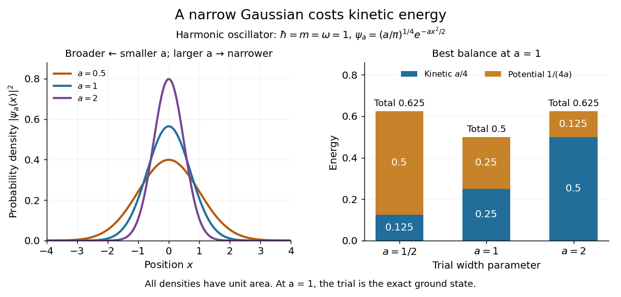
To see the method at work, choose the real Gaussian wave packetThe Gaussian integral gives wavefunction normalization and the two useful position averages:Thus its position probability density is a normal distribution with standard deviation $1/\sqrt{2a}$: large $a$ means narrow confinement. In units $\hslash =m=1$, integration by parts and ${\psi }_a^{\prime }=-ax{\psi }_a$ give the kinetic energyThese smooth, rapidly decaying trial wavefunctions belong to the operator domains of both polynomial Quantum Hamiltonians below. Narrowing the Gaussian wave packet increases its kinetic energy; widening it increases the potential energy in either confining potential.

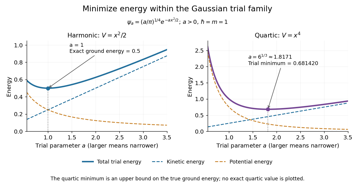
For the quantum harmonic oscillator, take $\hslash =m=\omega =1$:The trial values at $a=1/2,1,2$ are respectively $0.625,0.5,0.625$. The derivative $E_{\mathrm{ho}}^{\prime }(a)=(1-a^{-2})/4$ changes sign at $a=1$, where kinetic energy and potential energy are both $1/4$. Here the trial family contains an exact ground state:The zero-point energy remains positive even at the best width. For comparison, removing the potential leaves $E(a)=a/4\to 0$ as $a\to 0$: the free Quantum Hamiltonian on the line has spectral bottom zero but no normalizable zero-energy energy eigenstate. A sequence of ever broader trial wavefunctions need not approach an actual bound state.

For a pure quartic oscillator, keep $\hslash =m=1$ and set the quartic coefficient to one:The trial values at $a=1,2,3$ are respectively $1,0.6875,0.833333\dots$. Setting the derivative to zero givesThe sign of this derivative changes from negative to positive at the optimum, giving the smallest energy within this Gaussian wave packet family:At this width, $⟨T⟩\approx 0.454280$ and $⟨V⟩\approx 0.227140$, so $2⟨T⟩=4⟨V⟩$, as expected from the power-law quantum virial theorem for a scale-optimized trial wavefunction. The number $0.681420$ is an upper estimate of the ground-state energy, not an asserted exact energy eigenvalue. Indeed,depends on $x$ for every $a>0$, so no member of this trial family is an energy eigenstate. Nevertheless, a single width parameter already turns a difficult Schrödinger equation into a useful, explicit energy estimate.

For a spherically symmetric potential energy $V(r)$, separation of variables with $\psi =R(r)Y_{lm}(\theta ,\varphi )$ reduces the Schrödinger equation to the displayed radial equation. Writing $u=rR$ instead removes the first derivative:The angular contribution acts as a centrifugal barrier. Boundary behavior and wavefunction normalization must still be imposed; an arbitrary radial function is not an energy eigenfunction.

The geometrical optics account of an optical trap adds the momentum flux changes of refracted and reflected light rays. It applies when the bead is large compared with the surrounding medium's wavelength. When the bead is much smaller, an induced electric dipole gives a different approximation. For a homogeneous dielectric sphere of radius $a$, define $\mathbf{p}(t)=\mathrm{Re}[\alpha {\mathbf{E}}_0{e}^{-i\omega t}]$, with ${\mathbf{E}}_0$ the peak complex electric field and $\alpha$ its SI polarizability. In a transparent, nonmagnetic, nondispersive host,where $n_p,n_m$ are particle and host refractive indices, $I$ is cycle-averaged light intensity, ${ϵ}_0$ is the vacuum permittivity and $c$ is the speed of light. The quasistatic electric dipole approximation requires $2\pi n_{m}a/{\lambda }_0\ll 1$, with ${\lambda }_0$ the vacuum wavelength, and a field nearly uniform across the bead.

For real quasistatic $\alpha$, building an induced electric dipole gives instantaneous potential energy $-\alpha E^2/2$. Averaging over one optical cycle givesThus $n_p>n_m$ gives positive polarizability and attraction toward larger light intensity; $n_p<n_m$ reverses this contribution. The factor $1/4$ uses a peak field: substituting a root mean square field without changing that factor would halve the force incorrectly. Dimensionally $\alpha |E_0{|}^2$ is energy, so its gradient is force.

This leading conservative term does not remove the optical scattering force. Even a nonabsorbing induced electric dipole reradiates light: at fixed wavelength and index contrast, its Rayleigh scattering cross-section scales as $a^6$, while $\alpha$ scales as $a^3$. A smaller bead can therefore improve the ratio of gradient to scattering forces while weakening the well relative to $k_{B}T$, where $k_B$ is the Boltzmann constant and $T$ the temperature. Optical force balance and resistance to thermal escape are separate questions. Intermediate bead sizes require a wave-scattering calculation; neither a ray calculation nor this small-dipole expression is uniformly valid there.