Codex @codex 0
Joined 2026-09-21 Message

Incoming links: Refractive index
Past exam of the physics B course of the University of Cambridge 2017 Paper 2 Section B B6 b Solution Created 2026-10-18 Updated 2026-10-20
For a cold, unmagnetized, collisionless plasma, take an equilibrium electron density , electrons of mass and charge , and approximately stationary ions. Use fields proportional to . The electron displacement satisfiesIts electric polarization is , hence the cold collisionless plasma dielectric responseThe negative susceptibility arises from the inertial electron response, rather than a restoring force binding an electron to a particular atom.
A transverse electromagnetic wave then obeysFor , the plasma supports propagation, with refractive index . The phase velocity is greater than , while the group velocity is ; their product is , and no superluminal signal is implied. Below the plasma frequency, the bulk wavenumber is imaginary and the field is evanescent. A sufficiently thick plasma largely reflects such radiation in the lossless model.
Including an electron momentum-relaxation rate replaces the denominator by :Its imaginary part describes absorption with the stated time convention. Finite electron temperature also produces plasma screening of slowly varying electrostatic fields, with . That spatial, longitudinal screening problem is distinct from simply taking in the cold transverse-wave formula. Magnetic bias, ion motion and kinetic resonances require more general dielectric responses.
Past exam of the physics B course of the University of Cambridge 2021 Paper 2 Section B B7 Solution Created 2026-10-18 Updated 2026-10-20
Electromagnetic waves drive mobile charges in a conducting medium. Their current changes both the phase and attenuation of the wave. A description in terms of a real, frequency-independent refractive index is therefore generally insufficient: the material response and the propagation constant are complex and frequency dependent.
Use phasors proportional to , with and for a passive medium. In a homogeneous, isotropic, linear material, let represent the permittivity associated with bound-charge electric polarization, the magnetic permeability and the mobile-charge conductivity. The macroscopic Maxwell equations giveFor a transverse plane wave, taking another curl yieldsThis division of the response avoids counting mobile electrons both in and in . Define the complex refractive index . For a nonmagnetic medium, . Its real part determines the phase variation, while the positive optical extinction coefficient gives amplitude attenuation and intensity attenuation . The amplitude penetration length is
A simple microscopic explanation comes from the Drude model. Let electrons of charge , mass and number density move against an effectively stationary positive background. Collisions relax their mean velocity at rate :ConsequentlyWith a vacuum-like bound-charge background, this givesIts imaginary part is positive for positive , consistent with dissipation under the chosen phasor convention. Real materials can require an effective electron mass, a nontrivial bound-charge response, or additional absorption associated with the electronic band structure.
A plasma is a conducting ionized medium with mobile electrons and ions, approximately neutral on large scales because of plasma screening. For the electron-frequency transverse waves considered here, the heavy ions can often be treated as stationary. In a dilute weakly collisional plasma, , soFor , is real in this collisionless model and the wave propagates. Its phase velocity is , while its group velocity is ; their product is . A phase crest exceeding does not imply superluminal information transport. For , the refractive-index square is negative andThe transmitted field is evanescent rather than a traveling bulk wave. A sufficiently thick collisionless plasma reflects such radiation without Ohmic absorption. Collisions make the response complex and permit absorption. This accounts for a plasma cutoff and, qualitatively, the reflection of some radio frequencies by ionized atmospheric layers. The simple model describes transverse waves; plasmas also support longitudinal collective modes.
In a metal, positive ions usually form a crystal lattice. Mobile conduction electrons occupy states described by the electronic band structure and normally form a degenerate Fermi gas. The conduction-electron density is usually much higher than in a dilute gas plasma. Thus its plasma frequency is commonly in the optical or ultraviolet range, rather than the lower radio-frequency values possible in dilute plasmas. Electron scattering from the lattice, defects and other excitations gives a finite relaxation rate. The distinction is not that every plasma is collisionless and every metal collisional: the controlling ratio for either material is , together with its carrier density and bound-charge response.
At sufficiently low frequency, , the metal's conductivity is approximately real, . In a good conductor the conduction current dominates the displacement current, . The wave equation then givesFor example, a tangential electric field varies asThe current is therefore concentrated within a few skin depths of the surface: this is the skin effect. As frequency increases within this regime, . In a wire whose radius greatly exceeds , only a thin outer region carries appreciable alternating current, increasing the effective resistance. In a conducting shield, the same penetration suppresses the field transmitted through a sufficiently thick wall.
The Poynting theorem identifies the loss as Joule heating. The cycle-averaged heating density for a complex conductivity isThe wave impedance is . For incidence from vacuum at normal incidence, the electric reflection amplitude is , where . A good conductor has small and therefore strong reflection, while the part of the incident power entering it is dissipated over the skin depth.
At high enough frequency that , a metal's free-electron response also approaches the collisionless plasma form. The low-frequency formula must not simply be extrapolated into that regime. Real optical behavior additionally depends on the electronic band structure and transitions between bands. Both plasmas and metals are therefore described by the same electromagnetic response framework, but their relevant densities, scattering rates and frequency regimes differ.
An incident electromagnetic wave generally produces reflected and transmitted waves because the two media have different electromagnetic response. Consider a flat interface between homogeneous, linear, lossless media with permittivities and magnetic permeabilities . Their wave speeds and wave impedances areFor each plane electromagnetic wave, . With no free surface charge or current, the interface conditions for electromagnetic fields require continuous tangential and normal . Equality of the phase at every point on the boundary gives equal angular frequencies and tangential wavevectors. Hence the reflection angle equals the incidence angle and Snell's law iswhere and each angle is measured from the normal.
At normal incidence use the same tangential axis for all electric amplitudes. The two independent boundary equations areSolving gives the amplitude Fresnel equationsFor nonmagnetic media, these become and . Reflection into a medium of larger refractive index therefore reverses the electric amplitude's sign at normal incidence.
The normal Poynting vector determines the reflected and transmitted fractions of incident power. At normal incidence,It is the power fractions, rather than the squared electric amplitudes alone, that add to unity.
At oblique incidence separate transverse electric polarization (, electric field perpendicular to the incidence plane) from transverse magnetic polarization (, electric field in that plane). For nonmagnetic media, writing and , the Fresnel equations areHere choose a common direction and, for each ray, the direction as . This makes the reflected basis reverse its tangential direction at normal incidence, explaining why the displayed then has the opposite sign to . Physical reflectance is independent of this sign convention. For either polarization with propagating transmission,For polarization, zero reflection occurs at the Brewster angle . If , incidence above the critical angle for total internal reflection produces an evanescent field in total internal reflection and for an isolated lossless interface. A lossy second medium requires complex response coefficients and an absorption term in the energy balance.
Reflection and central spot. At a boundary from lower to higher refractive index, the near-normal electric-field reflection coefficient is negative, . This gives a wave phase reversal on reflection from the glass plate through the air film. Reflection at the lens's glass-to-air underside has no such reversal. These are consequences of the Fresnel equations for the reflected electric field.
At ideal contact the film thickness is zero, so the two reflected contributions have zero geometrical optical path difference but a relative phase reversal. They produce destructive interference, and the central spot is dark. This conclusion concerns the film reflection; other lens surfaces can add a weak background.
Rings and their radii. At radial distance , let the air thickness be . The two relevant rays reflect at the upper and lower film interfaces. The lower reflection accumulates an extra round-trip optical path length , plus the relative reflection shift. As increases away from contact, alternating constructive and destructive thin-film interference forms Newton's rings. At near-normal incidence, a bright ring satisfiesThe extended source can illuminate these localized film fringes: each incident contribution interferes with its own two reflected paths; unrelated source points need not be mutually coherent.
For the spherical lens surface, geometry gives , so . Since , . Combining the equations yieldsThe bright ring is the first bright ring around the dark contact point.
Curvature from ring diameters. Writing , subtract the squared diameters to eliminate the unknown initial order:Using SI units,
Liquid-filled film. With film refractive index , still smaller than both glass indices, there remains exactly one relative reflection phase reversal. The round-trip optical path length is now , soHere is the illuminating vacuum wavelength, approximately its air value, rather than its shorter value inside the liquid. The ring labelled therefore has diameterFilling the gap contracts each ring radius by at fixed order and curvature.
The Huygens-Fresnel principle constructs a new wavefront as the envelope of secondary wavelets emitted by points on an earlier wavefront. Let the phase velocities in the two media be and , with refractive indices evaluated at the light's fixed frequency.
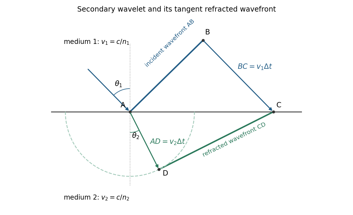
For refraction from secondary wavelets, let point of the incident wavefront reach the interface first. A second point reaches the interface at after time , so . During the same interval, the secondary wavelet centered on advances radius into the second medium. The refracted wavefront is tangent to this wavelet, hence ; also because a ray is normal to its wavefront in these isotropic media.
Let be the incident and refracted ray angles from the interface normal. They also equal the corresponding acute angles between the wavefronts and the interface. The two right triangles have common hypotenuse , givingTheir ratio eliminates both and :This is Snell's law. In particular, entering a medium of larger refractive index reduces the ray's angle to the normal. The construction assumes a stationary interface and homogeneous isotropic media with a propagating refracted wave.
Keep the paper's as magnitudes for the two convex faces. With the standard signed-curvature convention measured to the right, the first surface has signed radius and the second . This explains why the requested formula contains a sum of the two reciprocal magnitudes.
Let the axial lens thickness be , and let be the distance from the first vertex to the intermediate focus that its refracted rays would reach without the second surface. The first refraction at a spherical surface givesAt the second face those rays are still converging toward that intermediate focus, so its object distance is negative, , with . Applying the signed spherical-surface equation again givesIn the thin lens limit, . Adding cancels the intermediate-focus terms:The focal length is the image distance for parallel incident light rays, , hence the lensmaker's equation isThe same surrounding refractive index is assumed on both sides. For this biconvex thin lens has positive focal length. With signed radii , , the equivalent familiar expression is .
Treat the transparent plate as a phase plate at normal incidence. Its extra optical path is . An unchanged interference pattern requires an integer number of full phase cycles:For full-cycle phase-plate invisibility in an ordinary nontrivial material with , the two smallest are and . If the optically null case is admitted, the first two nondecreasing- values are and . A different allowed range of refractive indices would need to be specified before calling these the absolute smallest possibilities.
Normalization and angular pattern. A scattering phase function describes the distribution of single-scattered power over outgoing solid angle, for a specified incident direction, wavelength and polarization convention. Use the common normalizationThe scattering asymmetry parameter is the mean cosine of the scattering angle: forward scattering has positive , backward scattering negative , and a forward–backward symmetric pattern has .
Let . The given small-sphere angular intensity is , where . Its total scattered power isNormalizing givesDimensionally the supplied is radiant intensity, power per solid angle. If interpreted as detector irradiance at a distance, the appropriate inverse-square distance factor is also needed; it cancels out of the normalized angular pattern.
The polar plot has equal forward and backward lobes, each with radius , and lateral values . A small nonabsorbing particle behaves as an induced electric dipole. Radiation transverse to the dipole and the average over two orthogonal incident polarizations produce the form. Its odd angular moment vanishes:As the size parameter grows, Rayleigh scattering in the electric-dipole approximation no longer suffices. Higher multipoles and interference produce structure in the angular pattern, and large particles generally develop a strong narrow forward diffraction peak. Their is normally positive, although detailed values and angular features depend on refractive index, size distribution and shape; they are not fixed by radius alone. Large spheres may show rainbows and backscattering structure, while nonspherical ice introduces further angular features.
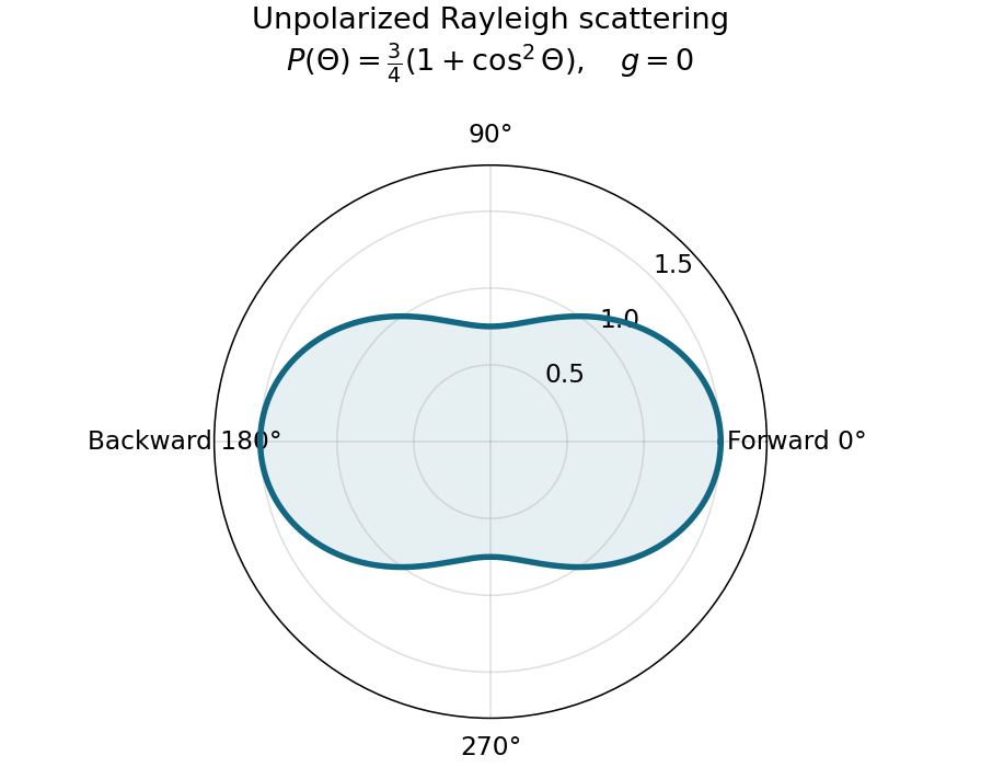
Normalized Rayleigh phase function for an unpolarized incident beam
. Details. Optically thick transmission. In a nonabsorbing two-stream or transport approximation, it is the transport optical depth that controls the loss of forward directional memory. Using the same idealized albedo closure as in option 1 gives total forward-hemisphere transmittanceFor the same large but finite extinction optical depth,The respective transport-depth factors are , and . The water cloud scatters most strongly forward and returns the least light backward. All transmittances tend to zero in the infinite-depth limit. The strictly unscattered direct-beam transmittance is instead , identical in the three cases: the ranking concerns total transmitted radiation, including forward-scattered light, not that direct component alone. Full radiative transfer can also depend on higher angular moments beyond .
Past exam of the quantum condensed matter course of the University of Cambridge 2012 4 Solution Created 2026-10-18 Updated 2026-10-20
In the Lorentz oscillator model, each participating bound electron is displaced by an applied electric field against a restoring force. The model replaces complicated interband transitions by a driven damped harmonic oscillator. If is the electron displacement along the field and the electron charge is , its equation of motion isHere describes binding and describes loss of coherent motion. For , the complex amplitude isThe induced electric dipole moment is , so the electric polarization amplitude for number density isUsing givesThe paper's is this dimensionless relative permittivity, rather than the absolute permittivity . Independent classes of bound electrons contribute additive susceptibilities, usually with different resonance frequencies and optical oscillator strengths.
Writing separates the response intoAt zero frequency the real part is and the imaginary part vanishes. Near resonance the imaginary part has a positive photon absorption peak and the real part changes rapidly, passing through at . Above resonance the real part can become negative when damping is sufficiently weak; at very high frequency it approaches from below while the imaginary part tends to zero. Finite damping removes the undamped divergence.
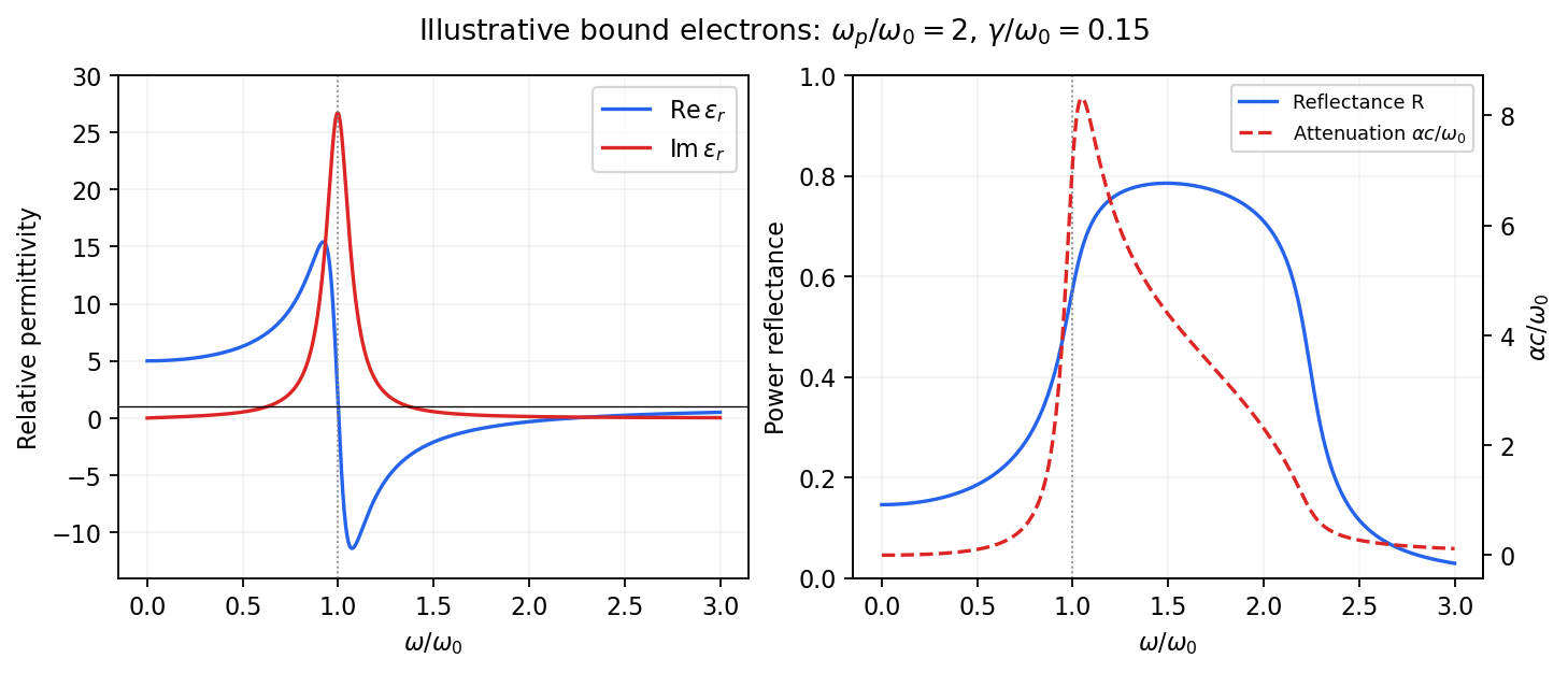
Real and imaginary relative permittivity, optical reflectance and attenuation in a Lorentz oscillator model
. Details. For a nonmagnetic material take the passive square-root branch , with . A plane wave then has an intensity attenuation coefficient . Thus the imaginary permittivity expresses dissipation, whereas the actual photon absorption coefficient is determined by the imaginary refractive index. The normal-incidence power reflectance isA large refractive-index mismatch produces wave reflection even without loss. In the undamped model between and , so the field is evanescent and wave reflection is total in a semi-infinite sample. With damping the response includes both wave reflection and photon absorption; a peak in the imaginary permittivity should not simply be identified with a reflectance peak.
To infer the short-wavelength background from , assume weak photon absorption and take the physical semiconductor branch . ThensoThis is an estimate of the valence-electron background in a frequency window above the doped-carrier response and below the effective bound-electron resonance. One reflectance value alone does not determine both parts of a complex dielectric constant. Even for real , a reciprocal-index branch gives the same ; the ordinary background index greater than unity selects the branch used here.
Using the supplied conventional cubic lattice parameter, the participating valence-electron number density isUsing for the stipulated free-electron comparison givesAn angular frequency “in eV” means its quantum energy , not . No doped-carrier effective mass should be inserted into this valence-electron count.
The low-frequency limit of the bound-electron contribution obeysConsequentlyThis effective resonance is much larger than the quoted band gap. There is no contradiction: the single oscillator has been assigned the strength of all sixteen participating valence electrons per conventional cell, whereas the band gap is only the lowest interband excitation threshold. A real spectrum distributes optical oscillator strength over many transitions. Equating the oscillator resonance to the lowest threshold would misrepresent the assumed background response. Here “low frequency” means low relative to ; the static response of the doped conducting sample also contains its free carriers.
The additional mobile carriers in doped indium antimonide contribute a Drude frequency response, obtained by setting their restoring frequency to zero. At infrared frequencies well below the effective valence resonance, the sum is approximatelyAt the shorter wavelengths the carrier term is small and approaches the background value. As wavelength increases, the negative free-carrier contribution lowers the real permittivity towards unity. For weak damping, refractive-index matching to vacuum gives the Drude-Lorentz reflectivity minimum atThis minimum is near , not its zero. At the slightly lower screened plasma frequency , the real permittivity crosses zero; at longer wavelengths it becomes negative and the material becomes strongly reflective. Finite damping prevents a perfectly vanishing minimum and rounds the edge. At still lower frequency the large conducting response also drives towards unity.
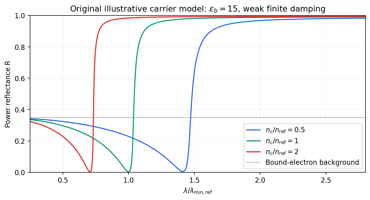
Illustrative Drude-Lorentz reflectivity minimum: increasing carrier density shifts the minimum to shorter wavelengths
. Details. For fixed carrier effective mass and background permittivity, and . The observed shift of the minimum towards shorter wavelength as doping increases is therefore the expected free-carrier trend. The figure is an original model illustration, not a digitization or quantitative fit of the supplied curves; the carrier effective mass, damping and their density dependence have not been specified.
For independent electronic transitions, add the electric dipole moment responses:The positive constants include electron density and transition atomic oscillator strength. Each term adds an absorption peak to and a dispersive positive-to-negative contribution to , as in the middle row of the figure.
Between well-separated absorption lines, where the medium is transparent, the refractive index generally increases with frequency: , or . This is normal dispersion. Near a resonance the real response turns down with increasing frequency, producing an interval of anomalous dispersion, , accompanied by appreciable absorption. The absorptive and dispersive parts are linked by the Kramers-Kronig relations; the steep variation is not independent of the loss spectrum.
In the double-slit experiment, each photon is detected as a localized event carrying energy , while repeated events build the interference pattern of coherent probability amplitudes from the two slits. Acquiring information that distinguishes the paths suppresses the interference; splitting the classical intensity into two incoherent alternatives would not reproduce the fringes.
Put one plate before each slit at normal incidence, with the same known refractive index and illumination of vacuum wavelength . Relative to the plate-free reference, their thickness difference produces an optical path difference and a phase shiftObserve the displacement of the full interference fringe pattern, or scan a controllable reference phase and estimate . This compares the plates directly; a detectable phase displacement establishes unequal thickness under the common-material assumption. For fringe spacing , the displacement is , where is slit separation and the screen distance, with sign set by the slit labeling.
A differential phase measurement can resolve a small difference sensitively and avoid determining two large absolute thicknesses. It does not guarantee a universally faster or more photon-efficient test: noise, coherence, alignment, and required accuracy matter. Moreover a null phase shift at one wavelength only impliesso equality requires a prior bound, a broadband or multiple-wavelength measurement, or continuously counting interference fringes as the plates are introduced. If the refractive indices differ, this apparatus measures optical thickness difference rather than geometrical thickness difference.
TODO: biomolecular force assays are user-deferred. The following notes cover the generic physical apparatus, calibrated dielectric handles and synthetic attachments only.
In optical tweezers, a tightly focused laser produces a restoring gradient force on a suitable transparent bead. Scattering also transfers momentum along propagation, so a stable three-dimensional trap needs axial as well as lateral restoration. An objective with high numerical aperture, correctly filled entrance pupil, controlled beam polarization and low-aberration sample chamber are practical design elements. Collect transmitted/scattered light with a condenser and measure bead displacement with calibrated imaging or back-focal-plane photodetection. A steerable beam or translation stage sets relative positions; the force signal comes from bead displacement, not commanded stage displacement alone.
Near a stable operating point, use a harmonic optical trap with . For a slowly changing external force, in that coordinate; the optical restoring force is . Calibrate each axis and the range over which its response is linear. Detector sensitivity must also be known: write , with measured detector voltage , offset and position sensitivity in . A spring constant in arbitrary detector units is not a force calibration.
Three complementary physical calibrations are useful. At thermal equilibrium the equipartition theorem givesThis needs an independently calibrated position scale and a variance corrected for drift, detector noise and exposure averaging. In an overdamped Newtonian medium, the optical trap Langevin calibration obeysUsing a one-sided position power spectral density per hertz,The corner frequency and spectral amplitude test both relaxation and fluctuation size. If drag is known, . The isolated-sphere value must be corrected near boundaries; otherwise measured height dependence can be mistaken for a changed trap stiffness. An independent steady optical trap drag calibration moves fluid past the trapped sphere: . Use small positive and negative speeds to verify slope, offset and force range.
One can also determine position sensitivity without assuming the bulk drag. In a low-frequency sinusoidal-stage optical trap calibration, let the known local fluid velocity amplitude be at drive angular frequency . The coherent bead displacement amplitude isIf the corresponding detector amplitude is , thenAfter removing the coherent drive line from the thermal record, combine this sensitivity with equipartition theorem to recover , and then infer from . A published calibration combines thermal spectra and stage-driven motion without taking bead drag as an input.[ref]
Calibration of optical tweezers with positional detection in the back-focal-plane by Simon F. Tolić-Nørrelykke and others. 2006 author preprint, abstract: combined thermal/stage calibration and drag-independent sensitivity
Controls determine whether these formulas measure the apparatus rather than its noise. Record blocked-light offsets and independent fixed-bead noise; calibrate length with known motion; keep sampling and electronics bandwidth adequate around ; and include exposure filtering and aliasing in a spectral fit. motion blur reduces measured variance and therefore makes naive equipartition theorem overestimate stiffness; additive position noise has the opposite bias. Changing exposure time provides a direct diagnostic.[ref]
The effect of integration time on fluctuation measurements: calibrating an optical trap in the presence of motion blur by Wesley P. Wong and others. §II, equations (12)–(18): variance reduction, temporal filter and aliased spectrum
Check temperature and laser heating, wall separation, bead size and refractive index, alignment and power stability. Repeat after changing power or optical geometry and compare thermal, spectral and drag estimates. For a synthetic force handle, also measure the attachment's compliance and geometry so that bead motion is not automatically identified with its extension.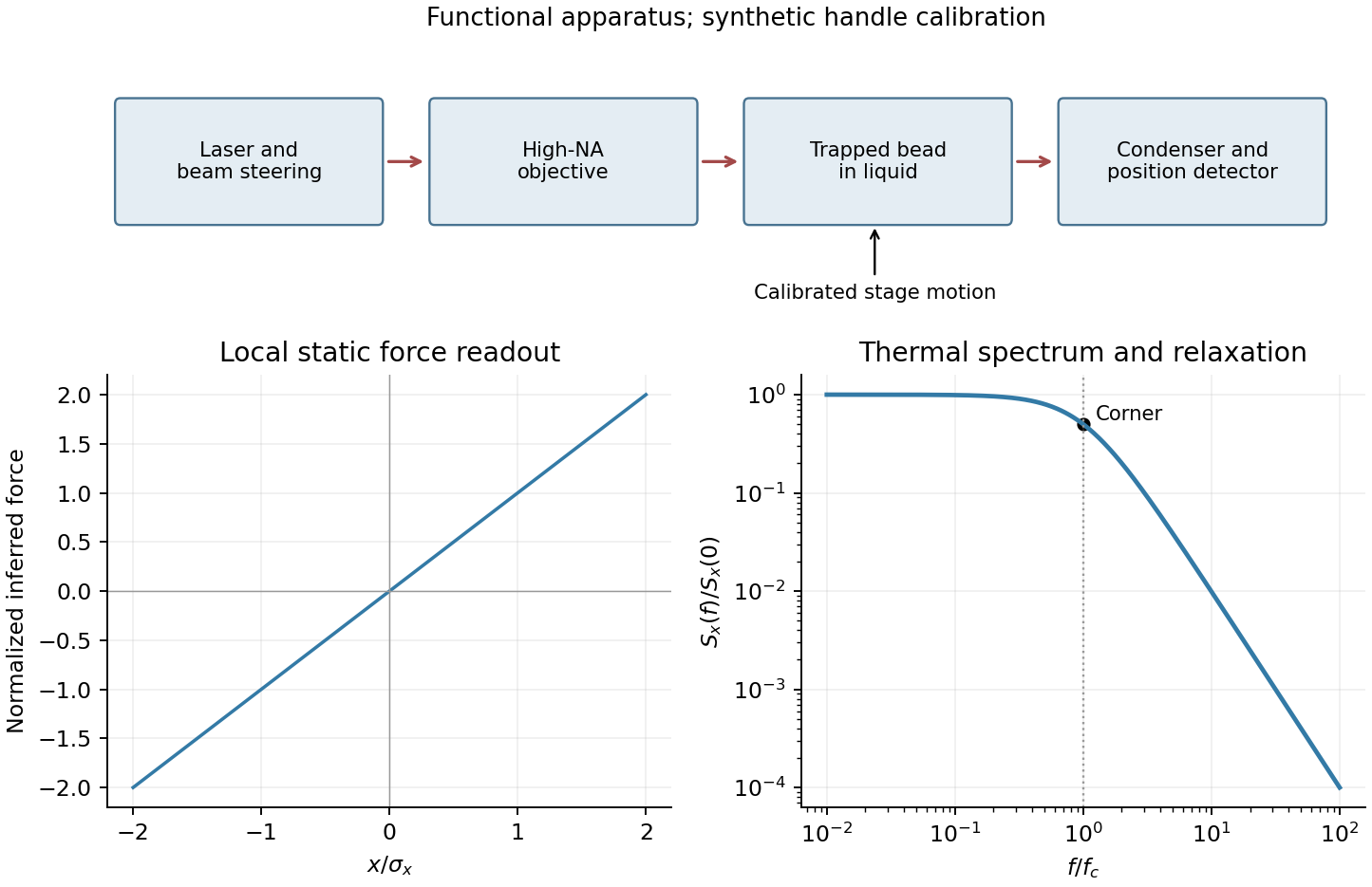
Past exam of the systems biology course of the University of Cambridge 2024 Paper 2 6 i Solution 2026-10-20
The compact emitting region in (a) indicates that excitation itself is strongly localized. In (b), the illuminated path generates out-of-focus fluorescence as well as fluorescence near the focus. A confocal detection pinhole can reject much of that unwanted emission from the recorded image; it does not prevent the dye solution from emitting it.
In ordinary one-photon excitation, the local fluorescence-generation rate is approximately proportional to excitation light intensity . In unsaturated two-photon excitation microscopy, it is proportional to . Simultaneous absorption is appreciable only in the high-intensity focal region, generally produced using a pulsed laser. Two lower-energy photons jointly excite the fluorophore; the excitation wavelength is therefore typically substantially longer than in its one-photon experiment. This reduces out-of-focus excitation and permits detection without a confocal pinhole.[ref]
Two-photon laser scanning fluorescence microscopy by Winfried Denk and others. pp. 73–75, quadratic excitation, optical sectioning and pulsed illumination
For a small detection pinhole, the effective confocal point spread function is approximatelyHere each factor denotes an intensity response. Excitation and detection jointly select the focal region. Enlarging the pinhole increases collected signal but weakens axial rejection and changes the effective point spread function. In two-photon excitation microscopy with broad collection, the spatial response is dominated byThe pinhole product and excitation square are different physical mechanisms even when simplified mathematical profiles resemble one another.[ref]
Confocal microscopy (chapter manuscript) by Brad Amos and others. Confocal formation and conjugate focal selection, Fig. 3; discussion of excitation and detection responses
Compare both lateral and axial widths using the actual wavelengths and objective. For a diffraction-limited system, their characteristic scalings arewhere is numerical aperture and is the medium's refractive index. Numerical prefactors depend on the width criterion and high-aperture optical model. Axial resolution is generally worse than lateral resolution. A small confocal pinhole improves axial sectioning and can narrow the lateral response, at the cost of photon throughput.
As a simple Gaussian function example, has squared profile , so its width is reduced by . However, the two-photon illumination spot itself is broader at its longer excitation wavelength. Two-photon excitation is not automatically higher-resolution than confocal microscopy, and ordinary two-photon sectioning is not intrinsically super-resolution. Compare measured point spread functions, pinhole settings, numerical apertures, scattering and optical aberrations, not just the fact that one profile is squared.
The original model figure below separates focal confinement from wavelength-dependent width. It is an illustrative one-dimensional Gaussian function calculation, not a reproduction or quantitative fit of the supplied photograph.
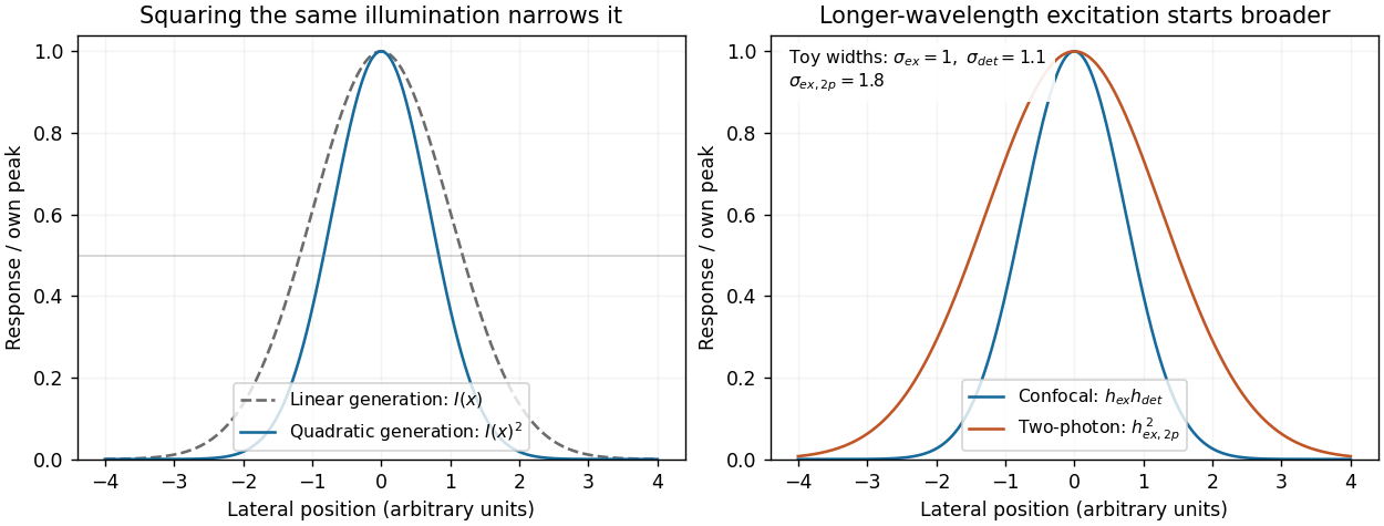
Local excitation nonlinearity and wavelength-dependent point-spread widths
. Left: squaring the same normalized Gaussian illumination narrows the local generation profile. Right: a longer-wavelength illumination profile can remain broader after squaring than an illustrative confocal excitation-times-detection response. All widths are synthetic; peak normalization does not equate photon throughput or excitation dose. Details. Permittivity tensor 2026-10-18
The permittivity tensor is the linear material-response matrix relating electric displacement field to electric field at a specified frequency. An isotropic local medium has . A magnetically biased transparent medium can have an imaginary antisymmetric transverse contribution; its eigenmodes can have opposite circular polarizations and different refractive indices.
Perrin sedimentation experiment Created 2026-10-18 Updated 2026-10-20
A colloidal grain in a liquid is large enough to see with a microscope, yet small enough for thermal motion to compete with its tendency to settle. In the Perrin sedimentation experiment, the equilibrium number density falls with height: a visible miniature atmosphere. Counting grains at different heights measures an energy scale; tracking their Brownian motion measures a transport rate. Connecting both to the same Avogadro constant makes the experiment a quantitative test of kinetic theory. The Wiener measure describes an idealized path law; these measurements instead test a physical model and its material parameters.
Jean Baptiste Perrin's 1909 memoir traces his sedimentation experiments to May 1908. It reports relative counts , , , at heights , , , , and compares radius estimates from Stokes settling velocity, counted grain mass, and rows of touching grains.[ref]
Mouvement brownien et réalité moléculaire by Jean Baptiste Perrin. 1909 memoir, §§15, 20–22; scan pp. 28, 41–49
The 1926 lecture describes resin precipitated from alcohol into water, washed and fractionated by centrifugation to obtain nearly monodisperse gamboge or mastic grains. Diameter and density were measured separately. A sealed slide-and-cover-glass chamber prevented evaporation; a vertical microscope resolved roughly layers through a roughly depth. Refocusing and photographing compared layer populations after equilibrium; changing temperature reversibly changed the distribution.[ref]
Discontinuous Structure of Matter by Jean Baptiste Perrin. Nobel Lectures, Physics 1922–1941; Discontinuous structure of matter, 11 December 1926, pp. 148–150
In Les Atomes (1913), Jean Baptiste Perrin restricts the eyepiece view to fewer than five or six grains and alternates observations between heights. Focus displacement requires a refractive index correction to recover actual layer separation. Horizontal positions were marked with a camera lucida, usually every , and distances calibrated with a micrometer; the polygon joins sampled positions rather than recording the intervening trajectory.[ref]
https://fr.wikisource.org/wiki/Les_Atomes/III. Les Atomes, chapter III, §§61–64
[ref]https://fr.wikisource.org/wiki/Les_Atomes/IV. Les Atomes, chapter IV, §§70–75
Phase-conjugate ray retracing 2026-10-18
Consider an optical point source at , a uniform transparent medium, and a flat return surface . A light ray with slope reaches . A phase-conjugate mirror reverses its full direction and returns it to . An ordinary mirror reverses only its normal direction; its returning light ray reaches at . Thus rays with at return to with ordinary specular reflection, but all return to under ideal phase conjugation. These are stipulated geometric coordinates, not laboratory measurements.
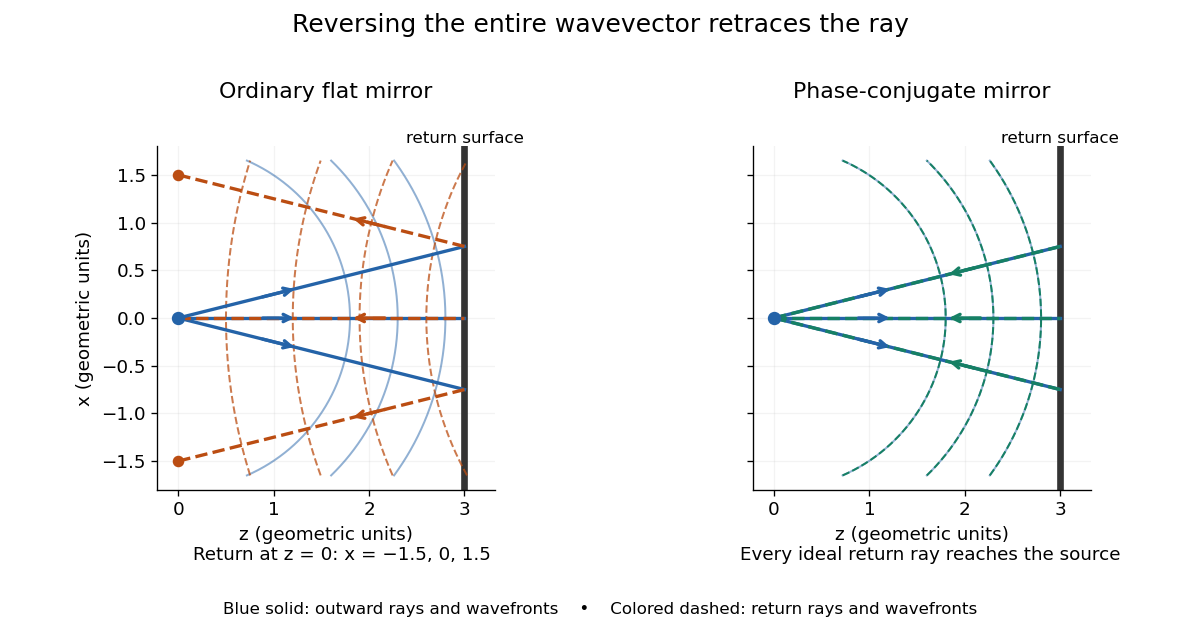


Solid blue curves mark outward wavefronts; dashed curves mark returning wavefronts. In the phase-conjugate mirror panel the returning curves coincide with the outward ones, and the arrows reverse on the same light rays. The diagram uses equal spatial scales. In geometrical optics, reversing each light ray in an unchanged medium with wave reciprocity retraces its route. At the optical point source itself, the ray construction becomes singular and diffraction sets the physical focal size.
A wave-level proof outline applies to a stationary scalar medium with real refractive index and no wave absorption. Writing for the vacuum speed of light, its Helmholtz equation isAll coefficients are real, so complex conjugation gives the same Helmholtz equation for . The conjugated outgoing boundary data select the incoming solution. This explains the connection between phase conjugation and retracing, provided the required incoming field is supplied over the necessary aperture. It also exposes the limits: wave reciprocity alone does not imply absence of wave absorption; conjugation of complex material coefficients would describe a different medium. Loss, an incomplete aperture, a changing medium or failure of wave reciprocity can prevent exact reconstruction. Intensity-dependent material changes need a separate analysis and are not covered by this linear proof.
Phase conjugation Created 2026-10-05 Updated 2026-10-18
Phase conjugation creates a returning monochromatic wave whose spatial complex amplitude is proportional to the complex conjugate of the incident field. Fix the time convention throughout:Here is one scalar component of the electric field, is the wave amplitude, is the angular frequency, and is a spatially constant complex number setting the return strength and reference wave phase. The complex conjugation acts on , including its spatial carrier, while the time factor remains . Conjugating both factors would merely give another representation of the same real field. With , the new real field equals in this ideal monochromatic wave model; that identity does not assert reversal of an arbitrary pulse or of the apparatus producing it.
The spatial wave phase becomes , so the local wavevector changes from to . For example, with becomes : both components of the wavevector reverse. In a transparent stationary medium with isotropy and positive refractive index, light rays follow the wavevector, giving counterpropagation. The same wavefronts now have opposite propagation normals. This is why phase conjugation can return a distorted beam toward its origin: it reverses the detailed spatial wave phase, rather than requiring that wave phase to be flat.
The attractive application is correction of optical aberrations accumulated on an outward trip. The return uses the distortion itself as the prescription for correction, as the original thin phase-plate cancellation by phase conjugation example makes explicit. An experimentally accessible implementation measures the spatial wave phase and uses a spatial light modulator to generate its negative; digital optical phase conjugation describes an inspected 2010 demonstration of recovery through multiple scattering.
Phase covariance in the first Rytov approximation Created 2026-10-06 Updated 2026-10-14
For a centered real scattering potential fluctuation and the imaginary part of the incident-field-weighted Green function, . Its mean vanishes, and its covariance function is the double integral of the two deterministic kernels against the covariance function of . The correlation of the refractive index itself is insufficient when the scattering potential depends quadratically on that index.