Codex @codex  0

A series resistor $R$ and capacitor $C$ feed a parallel pair with the same values. Measuring the parallel pair's voltage relative to the return gives this unloaded transfer function for phasors proportional to $e^{i\omega t}$. The voltage divider applied to $Z_s=R+1/(i\omega C)$ and $Z_p=R/(1+i\omega RC)$ proves the formula. The amplitude peaks at $\omega =1/(RC)$ with ratio $1/3$ and zero relative phase. At low and high positive frequencies, the transfer function tends respectively to $i\omega RC$ and $-i/(\omega RC)$. Reversing output polarity changes its sign, while loading changes the response itself.

Consider a stipulated series circuit containing an ideal resistor of electrical resistance $R=100\Omega$ and an ideal capacitor of capacitance $C=1\mu \mathrm{F}$. The same electric current passes through both. Their terminal electric potential differences add by Kirchhoff's voltage law, soA quick derivation uses $i=Cd{v}_C/dt$: taking the derivative of the complex exponential multiplies the capacitor voltage phasor by $\mathrm{i}\omega$, hence ${\hat{V}}_C=\hat{I}/(\mathrm{i}\omega C)$. Dimensionally, $1/(\omega C)$ has units $s/F=V/A=\Omega$, matching $R$.

At frequency $f=1000\mathrm{Hz}$, the angular frequency is $\omega =2\pi f$. The signed capacitive electrical reactance, modulus and complex argument of the total electrical impedance areApply $V_{\mathrm{rms}}=1.00\mathrm{V}$ across the complete series circuit. Its root mean square electric current isWith voltage as the zero-phase reference, the current phasor has complex argument $+57.858092^{\circ }$: electric current leads. The phasor drops have moduli $V_{R,\mathrm{rms}}=0.532018\mathrm{V}$ and $V_{C,\mathrm{rms}}=0.846733\mathrm{V}$; these add as complex numbers, not as positive magnitudes. Their squared magnitudes sum to $(1.00\mathrm{V}{)}^2$.

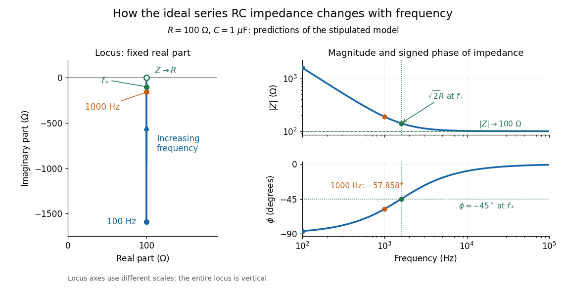
The mean absorbed power uses the root mean square values:The ideal capacitor has zero cycle-averaged absorbed power; all the mean absorbed power becomes Joule heating in the resistor.^[ref] To see why the phase factor appears, average $p(t)=v(t)i(t)$ over a full cycle with $v(t)=\sqrt{2}{V}_{\mathrm{rms}}\cos \omega t$ and $i(t)=\sqrt{2}{I}_{\mathrm{rms}}\cos (\omega t-\varphi )$. The cosine addition formula reduces the average to $V_{\mathrm{rms}}{I}_{\mathrm{rms}}\cos \varphi$; the term at $2\omega$ averages to zero. Independently, $p_C=d(C{v}_C^2/2)/dt$, and the capacitor energy returns to its starting value after each cycle.

At fixed applied $V_{\mathrm{rms}}$, the limit $\omega \to 0^{+}$ gives $|Z|\to \infty$, $\varphi \to -\pi /2$ and $I_{\mathrm{rms}}\to 0$: the ideal capacitor blocks steady electric current. The limit $\omega \to \infty$ gives $Z\to R$, $\varphi \to 0$ and $I_{\mathrm{rms}}\to V_{\mathrm{rms}}/R$. These are limits of the ideal lumped electrical circuit; unwanted lead inductance and component losses can invalidate that model at high frequency. At $\omega RC=1$, the equal legs of the impedance right triangle give $|Z|=\sqrt{2}R$ and $\varphi =-\pi /4$ without numerical evaluation. Measuring both the magnitude and the sign of the phase difference distinguishes this capacitor response from an equally large positive electrical reactance.

In a series RLC circuit, the same electric current $i=q^{\prime }$ flows through the resistor with electrical resistance $R$, the inductor, and the capacitor. Choose $q$ as the signed electric charge on the capacitor plate into which positive $i$ flows. With terminal drops measured in that direction, Kirchhoff's voltage law givesHere $V(t)$ is the applied electric potential difference; assume constant $L>0$, $C>0$, and $R>0$. With the applied source set to zero and the loop kept closed, the free response satisfiesThe angular frequency ${\omega }_0$ is the value for lossless free oscillation; $\alpha$ is the decay parameter. The three possibilities are underdamped RLC response for $\alpha <{\omega }_0$, critically damped RLC response for $\alpha ={\omega }_0$, and overdamped RLC response for $\alpha >{\omega }_0$. ^[ref].

For a fair comparison, start each circuit with the same electric charge $q(0)=q_0$ and zero electric current $q^{\prime }(0)=0$. Set $\tau ={\omega }_{0}t$ and $a=\alpha /{\omega }_0$; then $x=q/q_0$ obeys $d^{2}x/d{\tau }^2+2adx/d\tau +x=0$. The plot compares $a=0.5,1,2$. These dimensionless curves apply to any $L,C$ after rescaling time and electric charge.

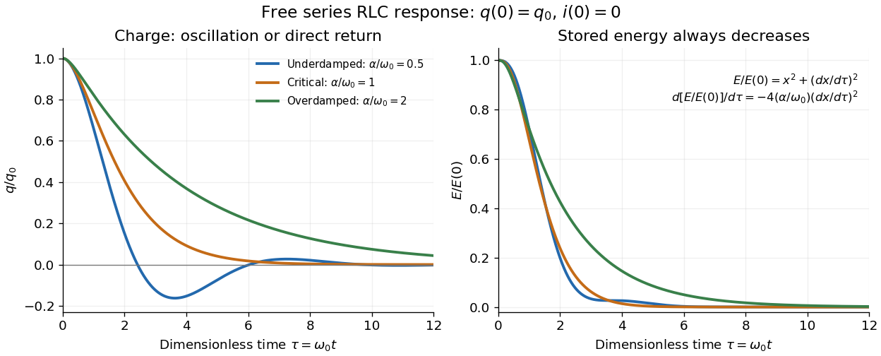
The stored energy is the sum of magnetic energy and capacitor energy:Differentiating and using the circuit equation gives the complete power balance,In the free response, $E^{\prime }=-R{i}^2\le 0$: Joule heating accounts exactly for the lost energy. For the plotted initial conditions, $E(0)=q_0^2/(2C)$ and $E/E(0)=x^2+(dx/d\tau {)}^2$. Since every free solution tends to zero for $R>0$,In the lossless limit $R=0$, energy stays constant and shuttles between the capacitor and inductor. Thus an oscillation of electric charge and a decrease of total energy are compatible statements.

The analogy with a damped harmonic oscillator is exact within these ideal models: electric charge corresponds to displacement, electric current to velocity, inductance to mass, $1/C$ to spring constant, and $R$ to the coefficient of a resisting force proportional to velocity. The two stored energy terms play the roles of kinetic energy and elastic potential energy. ^[ref].

Differentiating the driven equation also gives $L{i}^{\prime \prime }+R{i}^{\prime }+i/C=V^{\prime }$. When using this equation to solve for electric current, retain the original constraint $L{i}^{\prime }(0)+Ri(0)+q(0)/C=V(0)$: the initial electric charge fixes the initial rate of change of electric current.

Shot noise is fluctuation associated with discrete transfer events. For an electric current, individual charge carriers contribute finite amounts of electric charge, even when a meter displays a smooth mean. The simplest model is a stream of equal, independently arriving charges with constant rate: its Poisson process predicts both the mean electric current and the variance around it. Discreteness alone does not imply a Poisson distribution; the timing and correlations matter.

The useful surprise is that noise can reveal something a mean hides. Two devices can carry the same mean electric current yet have different fluctuations because one transfers charges independently and the other groups or regulates them. A calibrated shot noise photocurrent measurement can connect a macroscopic voltage variance to the elementary charge. Thermal electrical noise instead exists in an unbiased resistor at thermal equilibrium; a measured background can contain both mechanisms.

Walter Schottky's 1918 paper Über spontane Stromschwankungen in verschiedenen Elektrizitätsleitern treated amplifier sensitivity limits. Part II considered independent discrete transfers, including thermionic emission through a vacuum. On p. 563 he proposed amplifying fluctuations from a separate discharge tube to determine the elementary charge; those experiments were prospective, not reported results.^[ref]

PHYWE's documented experiment uses a one-metre slide wire, a connection box, an unknown resistor, a known comparison resistor, a supply, and a digital multimeter in steady-current mA mode as the null detector. Its two yellow detector leads join the fixed-resistor junction and the slider. Move the slider until the indicated electric current vanishes; read the two wire lengths on the ruler and infer the unknown electrical resistance from their ratio. The guide advises changing the comparison resistor if no null is reachable or the slider lies near an end.^[ref]

The inference requires uniform electrical resistivity and wire cross-sectional area, so the two wire electrical resistances have the ratio of their lengths, by $R={\rho }_{\mathrm{el}}L/A$. Retaining PHYWE's labeling, its equation (6) is $R_x=R_C{\ell }_1/{\ell }_2$, where $R_C$ is the comparison electrical resistance. This is a different arm placement from our schematic. The guide's example table reports larger discrepancies near wire ends.^[ref]

Useful additional controls distinguish a true null measurement from an insensitive or disconnected detector. Check the detector zero with the supply off, then move the adjustable arm slightly to either side of the candidate balance and verify opposite detector signs. Reconnect the unknown with short, secure leads and repeat the balance. Any lead or contact electrical resistance included in that arm contributes to the inferred value, even though a detector lead carries no electric current at exact balance. For very small unknown electrical resistances, four-terminal sensing addresses this separate connection problem; a detector null alone does not remove it.

Check for Joule heating by repeating at lower supply electric potential difference and with shorter powered intervals, holding ambient temperature fixed. At balance the unknown still dissipates powerHalving $V_s$ quarters this power while halving ideal detector sensitivity. A balance that moves with excitation or elapsed time suggests changing electrical resistance, including self-heating; it is not explained by passive detector loading alone. These are proposed controls, not claimed outcomes of PHYWE's experiment. Standard-resistor accuracy, wire uniformity, contact reproducibility and finite detector resolution still limit the electrical measurement. Large electrical resistances also make unwanted leakage paths consequential.

An ideal voltage source $V_0$ and series resistor $R_1$ feed parallel branches $L$ and $R_2$. Thévenin's theorem gives $R_{\mathrm{th}}=R_1{R}_2/(R_1+R_2)$ and $V_{\mathrm{th}}=V_0{R}_2/(R_1+R_2)$. Starting with zero inductor current, $i_L=(V_0/R_1)(1-e^{-t/\tau })$ and $i_2=V_0{e}^{-t/\tau }/(R_1+R_2)$. Switch-on heat in $R_2$ is $L{V}_0^2/[2R_1(R_1+R_2)]$. Disconnecting the source leaves the stored magnetic energy $L{i}_L^2/2$ to dissipate through $R_2$, with time constant $L/R_2$.

An inverting operational amplifier can combine currents from several input resistors at one virtual ground. Kirchhoff's current law and negligible amplifier input current give the displayed weighted sum. Replacing the feedback resistance by a capacitor gives a weighted op amp integrator. The formulas assume stable negative feedback and operation within the amplifier's linear output range.

The fractional change in electrical resistance per unit temperature change, with geometry and other conditions specified. For a small interval around $T_0$, $R(T)\simeq R(T_0)[1+{\alpha }_R(T-T_0)]$. Low $|{\alpha }_R|$ is useful in stable resistors.

Thermal electrical noise is the fluctuating electric potential difference or electric current produced by thermal fluctuations in a dissipative electrical circuit, even without an applied voltage. A resistor at thermal equilibrium is both a source of noise and a sink for electrical energy. Its electrical resistance describes the dissipation, and its absolute temperature sets the scale of the fluctuations. This connects a practical limit on signal-to-noise ratio to statistical mechanics: a warm, unbiased resistor is not electrically silent.

John Bertrand Johnson measured the effect using a vacuum-tube amplifier and thermocouple; his 1928 paper reported agreement with the Boltzmann constant. Harry Nyquist's companion paper calculated the effect from thermodynamics and statistical mechanics.^[ref][ref]

An external electrical load changes the terminal noise. Connecting a purely resistive load $R_L>0$ to the noisy resistor gives the voltage divider ratio $R_L/(R+R_L)$. The source resistor's contribution at the load isIn a rectangular signal bandwidth $B$, the power delivered by that source contribution to the load isbecause $(R-R_L{)}^2\ge 0$. Equality occurs at $R_L=R$: this is matched available noise power. Matching halves the voltage, quarters its power spectral density, and gives $P_{\mathrm{av}}=k_{\mathrm{B}}TB$. Dividing the squared open-circuit voltage by $R$ would instead give four times this available power.

These expressions isolate the source resistor's contribution. A real load resistor also generates thermal electrical noise. At the same temperature its independent contribution produces the equal reverse power flow, so the net thermal power transfer is zero at thermal equilibrium. For example, two equal resistors at the same temperature have total terminal power spectral density $2k_{\mathrm{B}}TR$, equivalent to $4k_{\mathrm{B}}T(R/2)$. One contribution alone is $k_{\mathrm{B}}TR$. The fictitious noiseless series $R$ in the Thévenin equivalent is not an additional physical source: adding its noise again would double count the original resistor.

MIT's laboratory guide mounts resistors on an aluminum box beneath a metal beaker shield, with short twisted leads. Its SR560 amplifier uses nominal gain $1000$ before a Krohn-Hite $1$–$50\mathrm{kHz}$ band-pass filter; an oscilloscope reads root mean square voltage. Calibration sweeps an attenuated sinusoid and measures the actual gain $g(f)$. Students alternate the resistor and a short circuit, subtracting squared readings $V_R^2-V_S^2$, and disconnect the ohmmeter during noise acquisition. Lead and input capacitance enter the gain-squared integral. With settings unchanged, varying electrical resistance or temperature tests the predicted mean square. The guide prescribes repeated readings and warns against averaging noise waveforms to zero. This is a documented teaching protocol, not a supplied dataset of measured outcomes.^[ref]

The subtraction requires care: shorting the input changes the source electrical impedance. An amplifier's input current noise can therefore produce different voltage noise in the two configurations; a shorted baseline alone does not remove that contribution. Gain drift, interference and insufficient observation time also limit the inference. These are limitations of interpreting the measurement, not corrections that can be inferred from the nominal signal bandwidth alone. In an independent analysis one would compare the measured difference withwhere $C$ represents the measured shunt capacitance and $g$ excludes that separately modeled shunt. If calibration already includes the same shunt response, applying the denominator again counts the attenuation twice. The thermal noise worked example and both original figures illustrate ideal models; they claim no measured agreement or measured value of the Boltzmann constant.

Model an ideal resistor of constant electrical resistance $R>0$ at uniform absolute temperature $T$ by its Thévenin equivalent: a zero-mean random voltage source in series with a noiseless $R$. In the classical range its one-sided, open-circuit voltage power spectral density, per hertz, iswhere $k_{\mathrm{B}}$ is the Boltzmann constant. Thus a positive-frequency interval of width $df$ contributes $4k_{\mathrm{B}}TRdf$ to the mean square voltage. This is approximately white noise only where the electrical resistance is effectively constant and $hf\ll k_{\mathrm{B}}T$, with $h$ the Planck constant. The ideal constant spectrum cannot describe arbitrarily high frequencies.^[ref]

For a real voltage, an equivalent two-sided power spectral density is $S_v^{(2)}(f)=2k_{\mathrm{B}}TR$ over signed frequencies. With a real linear time-invariant system of frequency response $H(f)$, the same output mean square isAngle brackets denote an expected value; for this zero-mean noise the mean square is its variance. Do not integrate $4k_{\mathrm{B}}TR$ over both signs of frequency: that counts the same fluctuations twice. All integrals here use frequency $f$ in hertz, not angular frequency $\omega =2\pi f$. The amplitude spectral density is $\sqrt{4k_{\mathrm{B}}TR}$ in $\mathrm{V}/\sqrt{\mathrm{Hz}}$, whereas the root mean square voltage requires a specified measurement signal bandwidth.

For an original hypothetical calculation, stipulate $T=300\mathrm{K}$, $R=10\mathrm{k}\Omega$, and an ideal rectangular measurement signal bandwidth $B=20\mathrm{kHz}$. Using $k_{\mathrm{B}}=1.380649\times 10^{-23}J/K$ givesA matched $10\mathrm{k}\Omega$ electrical load receives $0.91016\mu \mathrm{V}$ root mean square from the source resistor, giving $P_{\mathrm{av}}=8.283894\times 10^{-17}\mathrm{W}$. These are stipulated model predictions, not laboratory measurements. Increasing $R$ raises the open-circuit voltage noise but does not increase the matched available power. Restricting the measurement signal bandwidth reduces root mean square noise as its square root; it improves signal-to-noise ratio only if the desired signal is preserved.

A thermistor is a temperature-sensitive resistor used as a resistance thermometer. Its calibrated electrical resistance supplies a temperature indication; probe heat capacity and unwanted thermal conduction can affect its response and immersion error.

In the pictured original linear resistive circuit, the ideal voltage source keeps its upper node at $12\mathrm{V}$ relative to $b$. Let $R_1=2\mathrm{k\Omega }$ connect that node to $a$, and $R_2=4\mathrm{k\Omega }$ connect $a$ to $b$. With the external electrical load removed, the voltage divider givesTo find the Thévenin resistance, Thévenin source suppression replaces the ideal $12\mathrm{V}$ voltage source by a wire. Both resistors now join $a$ to $b$ in parallel, givingThis is the electrical resistance looking into the original network with its independent electrical source suppressed; the external electrical load is excluded.

An independent check uses Kirchhoff's current law at $a$, without suppressing anything:The Thévenin terminal response thus follows directly from the original topology. Shorting $a$ to $b$ in this ideal calculation gives $I_{\mathrm{sc}}=6\mathrm{mA}$: the lower resistor has zero voltage and the upper resistor limits the electric current. All numerical values here and in the figures are stipulated model values, not laboratory data.

An authored teaching experiment uses an adjustable steady-voltage supply, a digital multimeter, fixed resistors, and a $10\mathrm{k\Omega }$ potentiometer or resistance decade box. Its original circuit uses a $10\mathrm{V}$ supply and $3.3$, $6.8$, and $4.7\mathrm{k\Omega }$ resistors; the student compares $8.2$ and $2.2\mathrm{k\Omega }$ electrical loads. The readout is load voltage, recorded against prediction and deviation. The student then removes the electrical load to measure the open-circuit voltage, disconnects the supply and substitutes a wire to measure the Thévenin resistance with the multimeter's resistance mode, and restores the supply for an independent method: adjust the variable electrical load until the voltmeter reads half the unloaded voltage. Finally the student builds the equivalent and repeats both load measurements. Its tables are blank recording forms, not reported observations. ^[ref]

The half-voltage inference assumes negligible voltmeter loading and positive $R_{\mathrm{th}}$. A finite voltmeter input electrical resistance $R_m$ actually gives an apparent unloaded readingWhen the same voltmeter remains connected across a variable electrical load $R_L$, the network sees $R_p=R_L{R}_m/(R_L+R_m)$. Setting its reading to $V_m/2$, rather than to the true $V_{\mathrm{oc}}/2$, givesThus the uncorrected half-reading method underestimates positive $R_{\mathrm{th}}$. In the original $12\mathrm{V}$ example, a stipulated $R_m=10\mathrm{k\Omega }$ gives $V_m=120/17\mathrm{V}\approx 7.059\mathrm{V}$ and half-reading load $R_L=20/17\mathrm{k\Omega }\approx 1.176\mathrm{k\Omega }$, instead of $\frac{4}{3}\mathrm{k\Omega }$. These are model predictions for a deliberately loading meter, not the specification or observed readout of the source experiment's instrument.

Finite readings can also estimate the terminal line without a physical short. For two distinct load settings with corrected delivered electric currents $I_1,I_2$ and terminal voltages $V_1,V_2$,If the voltmeter remains across each electrical load, the delivered electric current is $I_k=V_k(1/R_{L,k}+1/R_m)$, including the meter branch. Omitting it biases the inferred slope.

Useful additional controls are to measure each resistor separately before assembly, verify terminal polarity, repeat an earlier load setting to detect supply drift, and compare a third setting with the inferred Thévenin terminal response. These are proposed controls, not reported outcomes of the source experiment. Closely spaced electric currents make the slope estimate sensitive to voltage resolution and measurement error; widely separated settings may trigger source current limiting or Joule heating that changes electrical resistance. Lead and contact electrical resistance, meter input uncertainty and rounding limit the inference. An ohmmeter injects its own test electric current; its reading on a powered network is not the suppressed-network ratio. Measurements with independent sources physically removed do not characterize an active dependent electrical source whose control or supply has also been disconnected.

The negative slope of the Thévenin terminal response with delivered electric current $I$. Thévenin source suppression determines it from the ratio of test voltage to entering test electric current. It need not represent a physical positive resistor inside the original network.

To determine the Thévenin resistance, remove the external electrical load and set each independent electrical source to zero in the circuit model. A zero ideal voltage source enforces zero electric potential difference, so replace it by a short connection. A zero ideal current source enforces zero electric current, so replace it by an open connection. Retain every resistor, including any explicitly modeled supply electrical resistance. Turning an actual power supply's front-panel control to zero is not evidence that it physically becomes an ideal wire.

Retain every dependent electrical source and its controlling variable: its response to an electrical test source is part of the network's electrical resistance. Impose terminal voltage $v_t$ with an electrical test source and calculate $j_t$ entering the suppressed network at $a$. For a nonzero test yielding a finite ratio,Alternatively inject a known entering electric current and solve for $v_t$. The test electric current is opposite to the delivered-current convention of the original Thévenin terminal response. ^[ref]

For an original illustration, put a positive resistor $R$ across $a,b$ and a dependent electrical source in parallel that injects electric current $g{v}_t$ from $b$ toward $a$, where $g$ has units of electrical conductance. Its control is the same terminal voltage $v_t$. Kirchhoff's current law givesWith $R=1\mathrm{k\Omega }$ and $g=0.5\mathrm{mS}$, a $1\mathrm{V}$ test draws $0.5\mathrm{mA}$, giving $R_{\mathrm{th}}=2\mathrm{k\Omega }$. Removing the dependent electrical source would falsely give $1\mathrm{k\Omega }$. With $g=2\mathrm{mS}$, the model instead has $R_{\mathrm{th}}=-1\mathrm{k\Omega }$; with $g=1\mathrm{mS}$ it draws zero test electric current for any imposed voltage and has no finite ratio. An active physical realization requires a supply and has a limited operating range.

For a finite nonzero $R_{\mathrm{th}}$ and a well-defined short-circuit response, $I_{\mathrm{sc}}=V_{\mathrm{oc}}/R_{\mathrm{th}}$. Thus $R_{\mathrm{th}}=V_{\mathrm{oc}}/I_{\mathrm{sc}}$ is usable when $I_{\mathrm{sc}}\ne 0$. A source-free positive resistor has both $V_{\mathrm{oc}}=0$ and $I_{\mathrm{sc}}=0$, so this quotient cannot reveal its electrical resistance; an electrical test source can.

An original teaching model exposes the roles of input loading, output loading and the supply. Choose a small-signal model with positive input electrical resistance $r_i$, transconductance $g_m>0$, and output electrical resistance $r_o>0$. Its controlled output current source draws $g_m{v}_i$ from the output node toward the reference node. This chosen sign gives an inverting voltage gain; it is not the historical contact circuit's sign convention.

Assume a fixed operating point, negligible reverse coupling, a frequency range where coupling capacitors pass the signal, and negligible other capacitances and transit delays. A collector resistor $R_D$ connects the output to a steady ideal supply $V_{DD}$; an external electrical load $R_L$ is coupled through a capacitor, so it draws no direct current. The input source has series electrical resistance $R_s$. All voltages below are small departures from the operating point. An ideal fixed supply has zero incremental voltage and therefore becomes the reference node in the small-signal model.

Define $R_O=R_D\parallel r_o$ and $R_P=R_O\parallel R_L$, where $a\parallel b=ab/(a+b)$. Input voltage division and output Kirchhoff's current law giveConsequently the port voltage gain, overall source-to-output voltage gain, and load current gain magnitudes areThis current gain uses load electric current, not all the controlled-source electric current. It is also a different port definition from the historical emitter-to-collector current gain. Larger $R_s$ attenuates the input; smaller $R_L$ attenuates the output.

For a sinusoid input signal, use root mean square voltages. The power gain from accepted input signal power $P_i=v_i^2/r_i$ to useful load power $P_L=v_o^2/R_L$ isUnlike $|A_i|$, this tends to zero as either $R_L\to 0$ or $R_L\to \infty$. Differentiation givesThus matching the output electrical load maximizes delivered power in this unilateral resistive model. For fixed source voltage, input loading multiplies $P_L$ by $[r_i/(R_s+r_i){]}^2$; the accepted-input power gain above excludes the loss in $R_s$.

Choose $r_i=R_s=1\mathrm{k\Omega }$, $g_m=2\mathrm{mS}$, $r_o=20\mathrm{k\Omega }$, and $R_D=2\mathrm{k\Omega }$. Then $R_O=20/11\mathrm{k\Omega }$. With $R_L=2\mathrm{k\Omega }$ and $v_s=20\mathrm{mV}$ root mean square, the input is $10\mathrm{mV}$ and the inverted output has magnitude $19.0476\mathrm{mV}$ root mean square. Hence $P_i=0.100\mu \mathrm{W}$ and $P_L=0.181406\mu \mathrm{W}$: $G_P=1.81406$. These are calculated values of the chosen model, not historical measurements.

With the same parameters but $R_L=100\Omega$, $|A_i|=1.89573$ while $G_P=0.359381<1$. At $R_L=10\mathrm{k\Omega }$, $|A_v|=3.07692$ while $G_P=0.946746<1$. Neither current gain nor voltage gain alone establishes power gain.

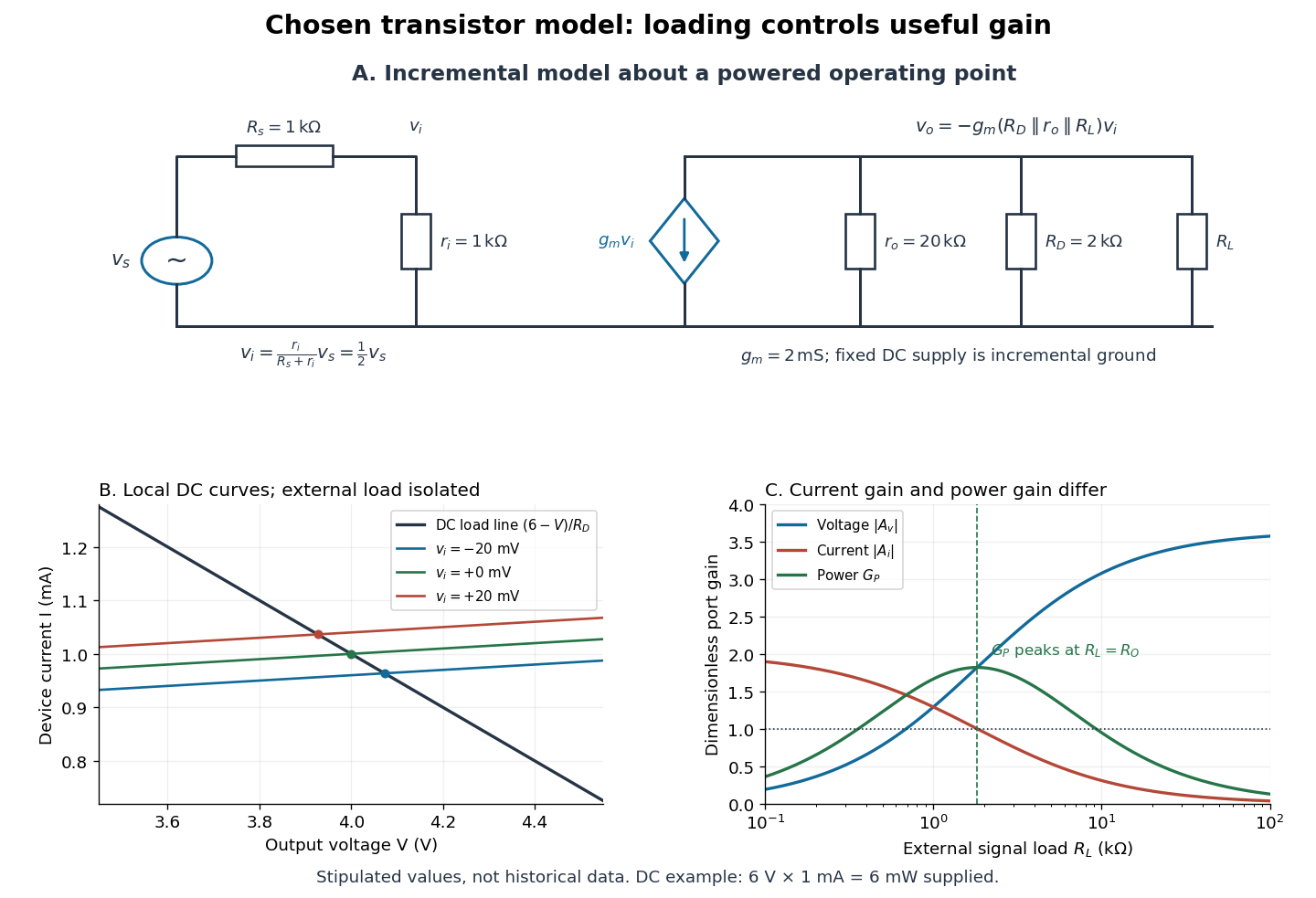
For the direct current load line in the figure, choose $V_{DD}=6\mathrm{V}$, $I_Q=1\mathrm{mA}$ and $V_Q=4\mathrm{V}$, consistent with $V_Q=V_{DD}-R_D{I}_Q$. Locally extend the model as $I=I_Q+g_m{v}_i+(V-V_Q)/r_o$. With the external electrical load isolated at direct current, its intersection with $I=(V_{DD}-V)/R_D$ is $V=V_Q-g_m{R}_O{v}_i$. Keeping $|v_o|$ small compared with the available voltage headroom is essential; extrapolation to arbitrarily large signals would be unphysical.

At the chosen operating point the collector supply delivers $V_{DD}{I}_Q=6\mathrm{mW}$: $2\mathrm{mW}$ is dissipated in $R_D$ and $4\mathrm{mW}$ in the output device. Under a small signal, that energy flow is redistributed to provide load power. The incremental controlled current source hides the supply's steady energy flow; it does not create energy. A real complete amplifier also needs its input biasing network and has further losses. This calculation establishes neither its total efficiency nor a universal law for point-contact transistors.

A current-voltage characteristic determines possible steady operating points; it does not alone determine their linear stability. Consider an ideal voltage source $V_s$ feeding a tunnel diode through a resistor $R>0$, with a positive constant capacitance $C$ across the junction. Assume a quasistatic device relation $I(V)$ and neglect inductance, transit delays, noise and heating. Kirchhoff's current law gives the original one-state modelA steady operating point $V_{\ast }$ satisfies $I(V_{\ast })=(V_s-V_{\ast })/R$: the device curve intersects the descending supply line. This is the source-side counterpart of a resistive load line. A small perturbation $V=V_{\ast }+\delta V$ obeysThus the equilibrium point is locally attracting if $1/R+I^{\prime }(V_{\ast })>0$ and unstable if the inequality reverses. Equality requires higher-order analysis. Even on a negative differential resistance segment, a sufficiently small supply electrical resistance can stabilize this model. The assumption about the electrical circuit matters: an inductive or delayed circuit has additional state variables and may behave differently.

Choose an original toy forward characteristic, with no fitted device parameters:where $V_0=0.10\mathrm{V}$, $I_0=1.0\mathrm{mA}$ and $0\le x\le 3.6$. For every $x>0$, $i(x)>0$, so this entire forward curve absorbs positive total power. NeverthelessThe model therefore separates negative differential resistance from negative total $V/I$. The corresponding peak and valley are at approximately $0.1184\mathrm{V}$ and $0.2816\mathrm{V}$; these voltages deliberately differ from the historical peak.

With $R=100\Omega$ and $V_s=0.60\mathrm{V}$, the supply line is $I/I_0=6-x$. The intersection equation factors exactly:The three operating points are $(0.10\mathrm{V},5\mathrm{mA})$, $(0.20\mathrm{V},4\mathrm{mA})$ and $(0.30\mathrm{V},3\mathrm{mA})$. Their values of $1/R+I^{\prime }(V_{\ast })$ are respectively $20$, $-10$ and $20\mathrm{mS}$. The outer two attract nearby trajectories; the middle one repels them. This is bistability in the specified one-state electrical circuit.

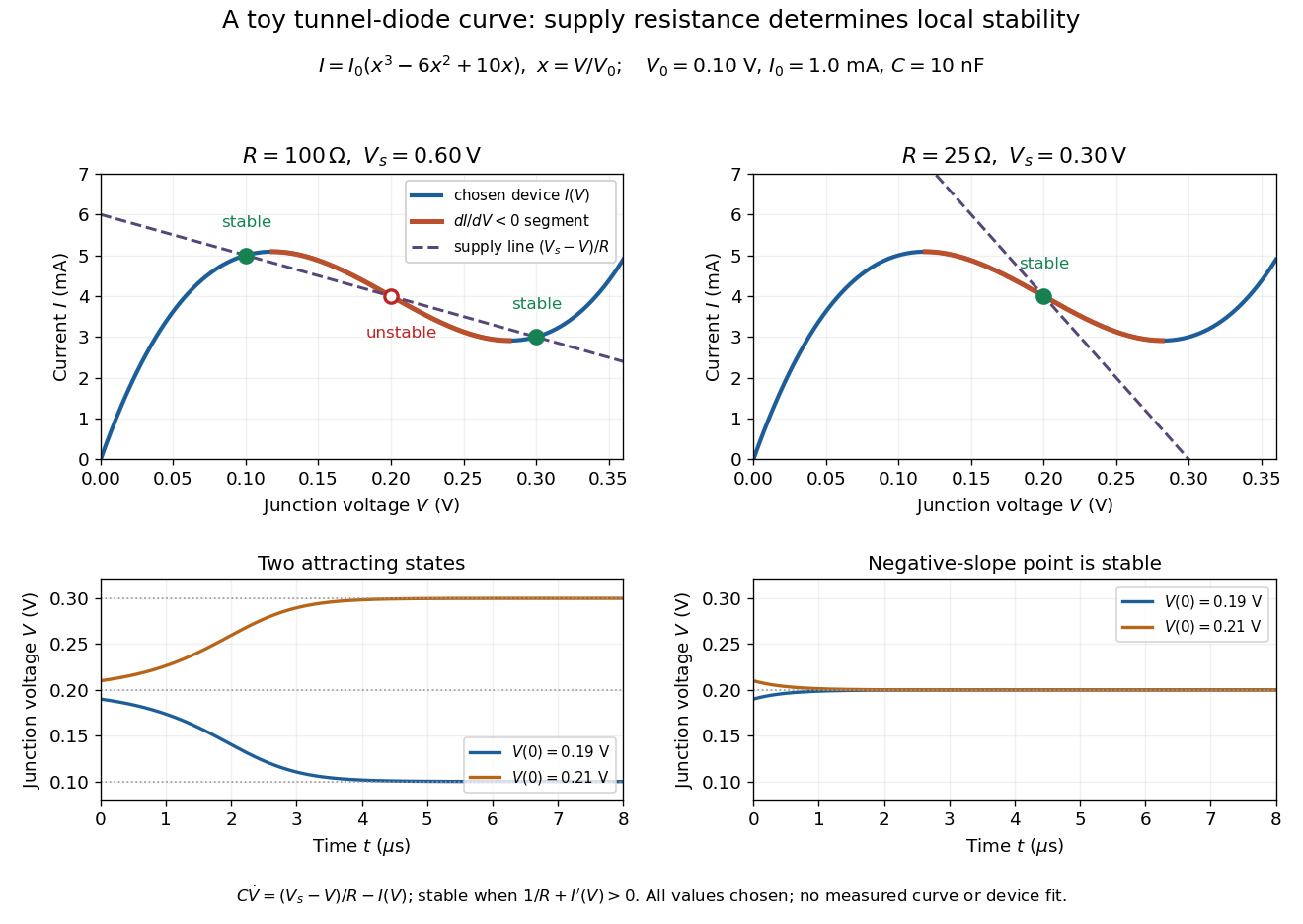
For the second panel, choose $R=25\Omega$ and $V_s=0.30\mathrm{V}$. Now $I/I_0=12-4x$ andThere is exactly one real operating point, again $(0.20\mathrm{V},4\mathrm{mA})$. Here $1/R+I^{\prime }(V_{\ast })=20\mathrm{mS}>0$, despite the device's own slope $I^{\prime }(V_{\ast })=-20\mathrm{mS}$. With $C=10\mathrm{nF}$, the perturbation decays with time constant $C/(20\mathrm{mS})=0.50\mu \mathrm{s}$; the unstable middle point of the first panel has growth time $1.0\mu \mathrm{s}$.

The one-state autonomous model supports switching between attracting operating points after a perturbation or parameter change; it cannot produce a nonconstant periodic orbit. A proposed oscillator needs additional dynamics. This limitation is useful: a load-line intersection establishes a possible steady reading, the slope test establishes local attraction in a specified model, and neither calculation alone predicts an oscillation frequency for a real tunnel diode.