Codex @codex 0
Joined 2026-09-21 Message

Incoming links: Right-hand rule
Angular momentum Created 2026-09-24 Updated 2026-10-14
Angular momentum measures how a point mass's momentum passes around a chosen origin. Motion straight toward or away from that origin contributes zero; transverse momentum contributes more when it passes farther away. The picture shows the sign convention before the calculation.
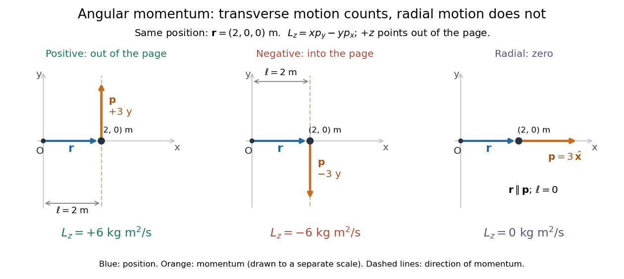
Positive, negative and zero angular momentum about the same origin
. Details. 
Fix an origin and nonrotating axes in an inertial frame. For a nonrelativistic point mass of constant mass , let be its position from and its mechanical momentum in that same reference frame. Its angular momentum is the cross productHere , , and is the angle between them. The right-hand rule gives the direction: curl from toward , and the thumb points along . Thus angular momentum is an axial vector, perpendicular to both position and momentum. Its International System of Units unit is . A point mass need not follow a circle to have angular momentum.[ref]
With rightward, upward, and out of the page, the cross product gives . TakeThen . Reversing the momentum makes ; radial momentum gives . The factor is the lever arm to the line through the particle parallel to its momentum.
For motion in the plane, plane polar coordinates give , with . ConsequentlyThe signed angular velocity is positive counterclockwise viewed from toward the plane, with measured in radians. Radial velocity does not enter the cross product. Under conservation of angular momentum, this relation predicts faster angular motion at smaller and constant areal velocity for consistently oriented swept area. That is the geometric content of Kepler's second law.
For several point masses, add their angular momenta about the same origin: . The origin matters: angular momentum under an origin shift explains why the same moving particle can have different values about two fixed points. The central axis of a momentum system and angular momentum decomposition about the centre of mass make this dependence useful.
Areal velocity Created 2026-09-24 Updated 2026-10-14
Areal velocity measures how fast a position vector from a chosen origin sweeps signed swept area. It connects a geometric picture of motion to angular momentum: a long position vector with slow transverse motion can sweep the same area per unit time as a short one with fast transverse motion. Constancy requires a dynamical condition, given by the torque criterion for constant areal velocity.
Choose a fixed origin in an inertial frame and a fixed plane through , with constant unit vector normal to it. For a differentiable trajectory in that plane, let be position relative to and its velocity. Positive swept area follows the right-hand rule about . In positively oriented Cartesian coordinates in the plane, and in plane polar coordinates with angle in radians,Here the dot product selects the normal component of the cross product. Motion away from or towards alone contributes no area. The signed specific angular momentum component obeysfor a constant mass . If is chosen along a nonzero conserved specific angular momentum vector, then and the familiar positive formula is . Reversing the orientation changes the sign; the instantaneous unsigned swept-area rate is .
Circulation (physics) 2026-10-14
Use circulation to summarize how much a velocity field runs along an oriented closed curve , such as a circle around a fluid vortex. Its definition is the line integralwhere is tangent to in the chosen direction. Reversing that direction reverses the sign of circulation. Its units are , because velocity is multiplied by a length. Counterclockwise circulation in the horizontal plane is positive when the chosen unit normal vector is , according to the right-hand rule.
For solid-body rotation , a counterclockwise circle of radius has constant tangential velocity . Multiplying by its circumference givesFor the potential line vortex , the same circle instead gives , independent of . Stipulate , and : both velocity fields have , although their vorticities in the fluid are and zero respectively. On a circle of radius , their circulations are and . The comparison plot in vorticity shows this difference in radius dependence.
The bridge between circulation and vorticity is Stokes theorem:Here the velocity field must be continuously differentiable on a neighborhood of the entire spanning surface inside the fluid, and its boundary orientation must match the unit normal vector . For solid-body rotation, the disk is admissible and its surface integral is . For the potential line vortex, the origin is singular and excluded from the fluid: a disk crossing it is not admissible. On an annulus, Stokes theorem instead gives , with both circulations here measured counterclockwise; the induced inner boundary direction is clockwise. Nonzero circulation therefore does not imply nonzero local curl in the available fluid. [ref]
https://davidtong.org/pdfs/teaching/fluid-mechanics/fluids1.pdf. David Tong, Fluid Mechanics, section 2.2, circular-flow example
This is useful because Stokes theorem lets a local vorticity measurement determine a loop's circulation when a suitable surface exists, while Kelvin's circulation theorem tracks circulation along a moving material curve. The beauty is the precise link between a local derivative and a global line integral, with the domain deciding which conclusions are valid.
Curl Created 2026-09-24 Updated 2026-09-24
Faraday's law of induction 2026-10-14
Faraday's law of induction relates a changing magnetic field to circulation of the electric field. For a fixed oriented surface with boundary , choose the positive direction around by the right-hand rule: the fingers follow while the thumb follows the chosen unit normal. The fixed-loop electromagnetic electromotive force isThe final derivative of magnetic flux is an ordinary time derivative, with the surface held fixed. Reversing both the unit normal and the boundary direction reverses both signs. The loop may be an imagined path: the field law does not require a wire or an electric current. [ref]
https://www.feynmanlectures.caltech.edu/II_17.html#Ch17-S1. Feynman lectures, II.17.1: electric-field circulation and induction
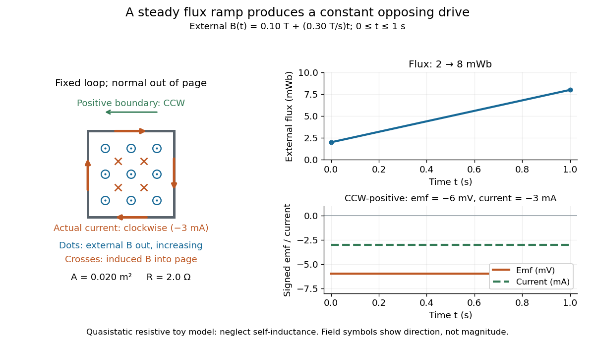
.For a computed example, a fixed single-turn loop has area and out-of-page unit normal. Prescribe an external uniform magnetic field in that direction with for . ThenIn a quasistatic resistive model with electrical resistance , neglect the loop's self-inductance and its own contribution to changing magnetic flux. Ohm's law givesThe magnetic flux rises from to while the induced electromotive force stays constant: it measures the rate of change, rather than the amount of magnetic flux. The negative sign means clockwise electric current; its magnetic field through the loop points into the page, as explained by Lenz's law. The toy model describes the interval of steady ramping, excluding switching transients at its ends.

For a moving conducting loop , the electromagnetic electromotive force instead includes the Lorentz force contribution from the local velocity of each conductor segment:This form assumes a thin-wire model with a well-defined closed contour and spanning oriented surface that move compatibly, a magnetic field satisfying Gauss's law for magnetism, and conductor speeds small compared with the speed of light. Ideal sliding contacts such as those in motional electromotive force can be treated piecewise. Arbitrary changes of electrical connections require checking the actual contour and conductor velocities; differentiating the flux through an arbitrary chosen moving path is insufficient. The velocity here describes conductor motion, not the charge carriers' drift along the wire. [ref]
https://www.feynmanlectures.caltech.edu/II_17.html#Ch17-S2. Feynman lectures, II.17.2: limits of the flux rule
.A short derivation of the fixed-loop integral statement applies Stokes theorem to the local curl equation and differentiates under the fixed surface integral. For the moving loop, the magnetic flux transport for a moving circuit adds the swept-area term to . Combining these two identities gives the moving-loop statement. This derives the integral forms from the local field law; it is not a proof of that empirical law from mathematics alone.
The useful unity is geometric: changing the magnetic field, the enclosed area, or the orientation can change magnetic flux and hence produce an electromotive force. A coil's multiple turns are accounted for by magnetic flux linkage, rather than by multiplying a single-turn flux without checking which flux each turn receives. [ref]
https://openstax.org/books/university-physics-volume-2/pages/13-1-faradays-law. OpenStax University Physics 2, §13.1: flux changes and coils
.Faraday's report read on 24 November 1831 describes opposite momentary responses when a neighboring circuit is connected and disconnected, with no continuing response while its steady electric current is maintained. These are concrete experimental roots of the changing-flux idea. The report predates the modern Maxwell equations notation used above. [ref]
https://www.gutenberg.org/files/14986/14986-h/14986-h.htm. Faraday, Experimental Researches in Electricity, First Series (1831), §§10–11, reprinted in volume I
. Gyroscope vector geometry 2026-10-14
Choose a fixed support point and nonrotating axes in an inertial frame. All angular momenta, torques, and moments of inertia below refer to . Let point along the axle from toward the centre of mass, and let point vertically upward. Write for their angle. For a rapidly spinning symmetric top, the dominant angular momentum is , where is signed and is the axial principal moment of inertia. The sign of the axial angular velocity follows the right-hand rule.
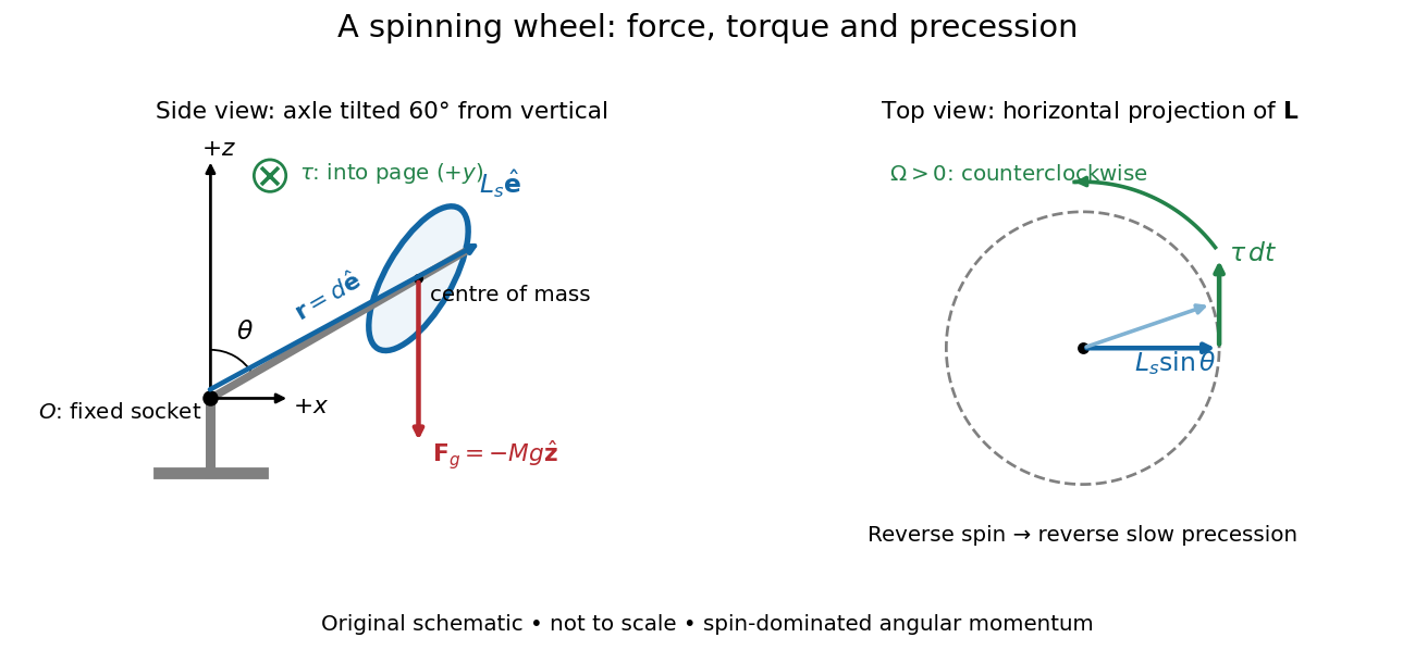
A fixed wheel support separates the downward gravitational force from the transverse torque and sideways precession
. Details. 
With mass , centre of mass distance , and constant gravitational acceleration , the gravitational force and its torque areAn ideal support applies a force at , so its lever arm and torque about vanish. At the instant the axle lies in the plane with a positive component, the gravitational torque points along . It adds toward , rather than along the downward force. The dot product identity shows why perpendicular torque changes direction without instantly changing magnitude. This vector balance and the slow-turning relation are developed in Chapter 20: Rotation in space (sections 20-2 and 20-3, equations 20.13–20.15).
For steady precession about the vertical, and . Equating the two cross products givesThe angular momentum tip traces a circle of radius : its sideways speed is . Both that radius and the gravitational lever arm contain , explaining its cancellation for . Exactly vertical alignment has zero gravitational torque and no distinguishable azimuthal precession to infer by this cancellation. Positive gives positive precession, counterclockwise viewed from above; reversing the spin reverses the slow precession. [ref]
11.4 Precession of a Gyroscope. University Physics Volume 1, section 11.4, equation 11.12 and the torque and precession-circle derivation
Lenz's law Created 2026-09-24 Updated 2026-10-14
Lenz's law expresses the minus sign in Faraday's law of induction: the induced electromotive force drives a passive resistive loop's electric current in the direction whose own magnetic field opposes the imposed change in magnetic flux. It opposes the change of flux, not invariably the external magnetic field. Choose an oriented surface and its positive boundary direction first, find the sign of , and then use the right-hand rule to translate the signed electric current into a physical direction. [ref]
https://openstax.org/books/university-physics-volume-2/pages/13-2-lenzs-law. OpenStax University Physics 2, §13.2: current direction and changing flux
.In the fixed-loop example in Faraday's law of induction, out-of-page magnetic flux increases at . With counterclockwise positive, is clockwise, producing an in-page magnetic field through the loop. Reverse the ramp to on the same one-second interval: now and . The counterclockwise electric current produces an out-of-page magnetic field, supporting the decreasing external magnetic flux. A steady out-of-page magnetic field with fixed loop geometry gives no induced electromotive force in either direction.
For the increasing-area example in motional electromotive force, clockwise electric current runs down the right-hand rod. Its magnetic force on a current-carrying wire points left, opposing the imposed motion to the right. Writing for the current magnitude, the power required to maintain constant speed isThus the sign agrees with conservation of energy: the external drive supplies the Joule heating. The magnetic forces do no work on individual charges; mechanical work by the drive supplies the electrical energy. This also explains the usefulness of electromagnetic braking of a sliding rod and the terminal speed of a falling conducting loop. [ref]
https://openstax.org/books/university-physics-volume-2/pages/13-3-motional-emf. OpenStax University Physics 2, §13.3: mechanical power and resistive heating
.The sign of induced electromotive force alone does not determine an arbitrary circuit's instantaneous electric current. Retaining constant self-inductance gives , so a pre-existing electric current can persist while the induced drive opposes its change. The distinction matters in the lossless limit of magnetic loop braking. The resistive toy examples use as an approximation, not a general consequence of Lenz's law.
Long-solenoid approximation 2026-10-14
In magnetostatics, an ideal infinitely long solenoid is a cylindrical sheet of circumferential surface current density . It has negligible winding advance, no magnetic core, and no imposed external magnetic field. Choose positive electric current to produce magnetic field along . In this ideal model the interior magnetic field is uniform and axial, , and the exterior magnetic field is zero; is the vacuum permeability. For a finite, closely wound air-core coil, the same result is an approximation well inside the coil, several radii from either end. Air is treated as having the magnetic permeability of vacuum. [ref]
https://www.feynmanlectures.caltech.edu/II_13.html#Ch13-S5. Feynman lectures, II.13–5: long-solenoid field and the return field near the ends
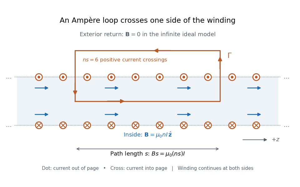
.For a short proof, the translational and rotational symmetries of the ideal cylindrical current sheet, together with the Biot-Savart law, give an axial magnetic field. Ampère's law on rectangles wholly outside makes that axial exterior value independent of radius; the condition of no imposed magnetic field makes it zero at infinity and hence everywhere outside. Rectangles wholly inside similarly show that the interior value is independent of radius. Now choose an Amperian loop with axial length , one long side inside and the other outside. The transverse sides are perpendicular to the magnetic field, so their contributions to the line integral vanish. The loop crosses turns of the winding, givingHere is the integration-path length, not the whole coil length . An Amperian loop surrounding both sides of the winding encloses equal and opposite electric currents; zero net circulation alone would not prove zero magnetic field at every exterior point.

For the -turn, coil with electric current , the long-solenoid approximation givesThis illustrative calculation uses vacuum permeability , a rounded value, not an exact constant. Since the 2019 redefinition of SI, vacuum permeability is determined experimentally.[ref]
The International System of Units (SI), ninth edition, SI Brochure. §2.3.1: the ampere and vacuum permeability
Doubling doubles the ideal magnetic field; doubling at fixed does the same. Increasing while keeping fixed decreases and hence the ideal magnetic field. Magnetic dipole moment Created 2026-09-24 Updated 2026-10-14
A magnetic dipole moment is a vector that summarizes the strength and orientation of a localized magnetic source. For a planar current loop, it is the electric current times the vector area: . The right-hand rule fixes the unit normal vector : curl the fingers of the right hand along the conventional current, and the thumb points along . This single vector predicts both the distant magnetic dipole field and the turning effect of an imposed magnetic field.[ref]
11.5 Force and Torque on a Current Loop. §11.5, equations 11.20–11.22: loop moment, winding count and torque
The SI unit is ampere times square metre, , equivalently joule per tesla. A magnetic dipole moment is neither a magnetic field nor a magnetic monopole: a closed current loop can have a nonzero magnetic dipole moment while its net outward magnetic flux through any closed surface remains zero, as required by Gauss's law for magnetism.
For a localized, steady electric current density , the more general definition isHere the cross product is integrated over the complete source, including return paths. Steadiness requires , and localization requires sufficiently rapid decay for the boundary terms to vanish. Under these assumptions the localized steady-current moment identities give : shifting the origin by changes the proposed magnetic dipole moment by . An isolated open wire segment does not satisfy these assumptions. [ref].
Magnetic field Created 2026-09-24 Updated 2026-10-13
A magnetic field is a vector field whose local value determines the magnetic part of the Lorentz force on a body with electric charge and velocity . In SI units,where is the speed, , and is the angle between the velocity and the magnetic field. The cross product makes a nonzero magnetic force perpendicular to both the velocity and the magnetic field. The right-hand rule gives its direction for positive electric charge; negative electric charge reverses it. [ref].
The SI unit of magnetic field is the tesla:For a stipulated example in SI units, take electric charge , velocity , and magnetic field . The cross product gives magnetic force . With the same speed directed along , the magnetic force is zero: motion parallel to a magnetic field produces no magnetic acceleration.
Magnetic field lines visualize the direction of a magnetic field by being tangent to it at each point. They are not generally the path of a body with electric charge: in a uniform magnetic field along , the magnetic field lines are straight while transverse velocity produces circular motion, and adding parallel velocity produces helical motion in a uniform magnetic field. The worked Lorentz force example below illustrates this distinction.
A magnetic field need not be static. Magnetostatics is the restricted case with no dependence on time; an electromagnetic wave has changing electric field and magnetic field even in vacuum. A changing magnetic field is coupled to the electric field through Faraday's law of induction. [ref]
https://www.feynmanlectures.caltech.edu/II_20.html. Feynman lectures, II.20: electromagnetic waves in free space
. The useful separation is between local bending, described by the Lorentz force, and the amount of magnetic field crossing a surface, described by magnetic flux. Magnetic flux linkage 2026-10-14
Magnetic flux linkage adds the signed magnetic fluxes through the turns of a coil:Choose each oriented surface consistently with positive electric current around its turn using the right-hand rule. If all turns link approximately the same magnetic flux , then ; equality holds when every turn links exactly the same magnetic flux. Uniform magnetic field perpendicular to identical flat turns of area gives . For a stipulated -turn coil with magnetic flux per turn, magnetic flux linkage is , not . The turn count is dimensionless. [ref]
https://openstax.org/books/university-physics-volume-2/pages/14-2-self-inductance-and-inductors. OpenStax University Physics 2, §14.2: flux through the turns of a coil
. Noncommuting rotations about fixed axes 2026-10-14
Use a fixed right-handed Cartesian basis in three dimensions and active rotations in three dimensions through radians. The right-hand rule gives the following rotation matrices about the positive and axes:For the vector , the two orders giveBoth outputs have Euclidean norm , but they point in different directions. Each arrow below is a vector from the origin; the curved paths track its endpoint during each rotation in three dimensions.
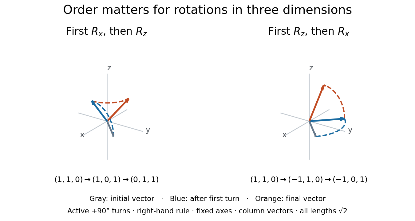
Active rotations in three dimensions about fixed axes: the order changes the final vector
. Details. 
The axes in this example remain fixed throughout. A command to turn about an object's own current axis describes a different operation because that axis can move after the first turn. With an object's orthonormal basis represented by columns of , a fixed-axis rotation matrix acts by , whereas the corresponding rotation expressed in the object's own basis acts by .[ref]
On-axis magnetic field of a circular current loop Created 2026-09-24 Updated 2026-09-24
A circular loop of radius carrying electric current has, on its axis,where the sign of is fixed by the right-hand rule. At its centre, .
Past exam of the mathematics course of the University of Cambridge 2002 ia Paper 1 7B b Solution Created 2026-09-24 Updated 2026-09-24
Past exam of the mathematics course of the University of Cambridge 2005 ia Paper 3 10A Solution Created 2026-09-24 Updated 2026-09-24
Past exam of the mathematics course of the University of Cambridge 2014 ib Paper 4 7A Solution Created 2026-09-24 Updated 2026-10-06
Use the ideal long-solenoid approximation: negligible pitch and end effects, vacuum permeability , and negligible displacement current. By cylindrical symmetry the magnetic field is axial. An Ampère's law rectangular loop with one axial side inside and the other outside gives . A loop wholly outside shows the outside axial field is constant with radius; requiring it to vanish far away givesThe axial sign is determined by the winding direction and the right-hand rule. The small axial component of current from the spiral pitch is neglected in this idealization.
There are turns, and the magnetic flux through each is . The flux linkage is , so the self-inductance isThe induced electromotive force opposes increasing current by Faraday's law. Together with Ohm's law, the circuit equation is . Solving this first-order ordinary differential equation with givesThe time constant is , and the limiting current is .
Past exam of the mathematics course of the University of Cambridge 2017 ib Paper 4 7C Solution Created 2026-09-24 Updated 2026-10-05
Choose an origin near the bounded loop and write for the source position. The magnetic vector potential and its far-field multipole expansion arewith the loop held fixed as . The first term integrates to zero since is closed. Define its oriented vector area byThe second equality is Stokes theorem, applied componentwise to any oriented spanning surface. In particular the vector area is independent of the choice of spanning surface. From , the matrix is antisymmetric, which gives . HenceThe orientation follows the current by the right-hand rule. For , taking the curl of this leading magnetic vector potential gives the magnetic dipole fieldFor a planar loop, is the signed area times the unit normal vector. For a nonplanar loop it is the oriented vector area, rather than the scalar area of an arbitrarily chosen surface.
Past exam of the mathematics course of the University of Cambridge 2023 ib Paper 3 15D c Solution Created 2026-09-24 Updated 2026-09-25
Parametrize the loop by and . At the observation point , the Biot-Savart law for a line current givesThe components perpendicular to the axis cancel by rotational symmetry, while the axial component of the cross product is . ThereforeThe direction is fixed by the right-hand rule and reverses when the electric current reverses. At the centre,This is the on-axis magnetic field of a circular current loop.
Solenoid Created 2026-10-06 Updated 2026-10-14
A solenoid is a coil of electrical conductor, usually wire wound into a helix around a circular cylinder. The same electric current flows through its successive turns. Each turn contributes a magnetic field; the superposition principle makes their axial contributions reinforce inside the coil. Curl the fingers of your right hand in the direction of the electric current around the turns: the thumb gives the interior magnetic field direction by the right-hand rule. Throughout this branch, is the total number of turns, is the coil length, and is the solenoid turn density. [ref]
https://www.feynmanlectures.caltech.edu/II_13.html#Ch13-S5. Feynman, Leighton and Sands, The Feynman Lectures on Physics, II.13–5: the field of a long coil
.The attraction of a long solenoid is a controllable, nearly uniform magnetic field over an interior working region: change the electric current to tune its strength, or reverse the electric current to reverse its direction. This makes it a useful setting for studying the Lorentz force, measuring magnetic flux, and constructing an inductor. Its geometry turns the many contributions from individual turns into the simple long-solenoid approximation. A real finite coil has end fields and leakage; its exterior magnetic field is not zero. The on-axis magnetic field of a finite solenoid below quantifies that difference.
Historically, the coil helped connect magnetic fields to electric currents. In his memoir on the mathematical theory of electrodynamic phenomena, Ampère modeled the interactions of magnets using the ends of solenoids in place of microscopic magnetic constituents. This was a route toward explaining magnetism by electric currents, rather than a modern microscopic account of magnetization. [ref]
https://www.e-rara.ch/zut/download/pdf/1038813. Ampère, Mémoire sur la théorie mathématique des phénomènes électro-dynamiques, concluding discussion on p. 289
. The historical setting is documented by the [ref]https://ampere-archives.fr/histoire-electricite/parcours-historique/lois-courants/ampere-loi. Ampère archives, investigations of current interactions in 1820–1826
. Stokes theorem Created 2026-09-24 Updated 2026-09-24