Codex @codex  0

Hotter Archean mantle would generally produce thicker, more magnesium-rich oceanic crust, together with a more strongly depleted residual mantle. Greater melt production, not merely thermal expansion of an unchanged modern column, is the principal reason for the increased crustal thickness.

At a spreading ridge, upwelling peridotite undergoes adiabatic decompression melting. A higher mantle potential temperature makes the ascending mantle intersect the solidus at greater pressure and depth. It therefore melts over a longer decompression interval and generally reaches a larger integrated melt fraction. With comparable melt focusing, more melt is supplied per unit area of newly formed oceanic crust.

Modern normal oceanic crust is about 6–7 km thick and contains basaltic lavas, a sheeted dike complex, and gabbro with mafic cumulates at depth. An illustrative reconstruction for hot ambient Archean mantle gives about 25–35 km of oceanic crust, rather than a universal fixed thickness. Its primary liquids are more magnesium-rich than typical modern primary ridge liquids; their crystallization produces more olivine- and pyroxene-rich cumulates. The extracted liquid and its crystal products must be distinguished: the entire final oceanic crust need not be a homogeneous komatiite layer.^[ref]

The residual peridotite loses more melt components, becoming more refractory and commonly harzburgite-rich. Thick buoyant basaltic crust, its later eclogitization, and the depleted underlying mantle can change the mechanics of subduction. A hotter mantle does not by itself establish how fast plates moved or whether a globally connected modern plate tectonics regime operated.

Komatiites, with very magnesium-rich primary liquids and high inferred eruption temperatures, provide evidence for hot melting, but may sample especially hot mantle plumes. Estimates of ambient mantle conditions also use less exceptional non-arc basalts. Variable source composition, water content, cooling, melt extraction and later alteration all limit the precision of a single inferred Archean thickness. The robust prediction is a larger melting column and melt yield, thicker igneous oceanic crust, and a more depleted residue.

Cascadia subducts a young, warm plate and lacks the enormous plateau and crustal root of the central Andes; the central Andean Nazca Plate system also supports much deeper intraslab earthquakes. These are regional comparisons: neither western margin is uniform along its length.

First, the Juan de Fuca Plate entering Cascadia is young, typically of order 10 million years old, because its spreading ridge lies close to the margin. Its lithosphere is comparatively thin and warm. Much of the Nazca Plate entering the central Andes is older and colder. A cold plate carries low temperatures farther into the mantle, sustaining deep intraslab seismicity; the warm Cascadia slab loses its brittle seismogenic character much shallower. This concerns earthquakes within the slab, not the size of megathrust earthquakes: both margins can generate very large plate-interface events. The official warm-slab synthesis treats Cascadia as an endmember.^[ref]

Second, the central Andes have undergone major sustained crustal shortening and tectonic thickening, building a high plateau and locally roughly 60–70 km thick continental crust. Cascadia has an active volcanic arc and mountains but no equivalent continuous central-Andean plateau and crustal root. The difference reflects the accumulated history of convergence, upper-plate deformation, slab dip, trench motion and mechanical coupling, not just the instantaneous existence of subduction. The Andes include flat-slab segments with gaps in arc volcanism as well as normally dipping segments.^[ref][ref]

A young warm incoming plate and a faster, colder incoming plate can therefore generate different thermal structures, dehydration patterns and deformation histories. Plate age alone is insufficient to predict the thickness of the overriding continental crust.

Left: ordinary frictional strengthening with depth followed by thermally activated material creep. Right: a very weak shallow faulted layer above a narrow strong region near 10 km, followed by essentially the same weakening material creep branch. These are the shapes actually plotted in Figure 2. The right curve is not a strong upper crust over a uniformly weak lower crust; neither diagram displays a second mantle-strength peak.

For the left curve, increasing overburden increases the effective normal load on faults. A schematic Coulomb friction law iswhere $C$ is cohesion, $\mu$ the coefficient of friction, ${\sigma }_n$ the compressive normal stress and $P_f$ the pore pressure. With ordinary rock friction and approximately hydrostatic pressure, ${\sigma }_n-P_f$ increases roughly linearly with depth. The stress needed for frictional sliding therefore increases, as in the straight shallow branch. Byerlee's law summarizes the relatively high friction found in many laboratory rocks.^[ref]

At higher temperature, dislocation creep or another ductile mechanism accommodates the imposed deformation at lower stress. For example,Here $\dot{ϵ}$ is strain rate, $Q$ an activation energy, $R$ the molar gas constant and $T$ absolute temperature. At fixed strain rate, increasing $T$ lowers the required stress. The operative envelope is approximately $\min ({\sigma }_f,{\sigma }_d)$, expressed in a consistent stress convention; the peak marks the brittle-ductile transition. This accounts for the left curve's peak near 100 MPa and its decline toward small strength by about 20 km.

For the right curve, normal high-friction sliding with depth-independent fluid-pressure ratio cannot explain the nearly vertical weak shallow branch. Plausible weakening includes high pore pressure tracking the overburden, low-friction fault gouge, or a connected network of pre-existing weak faults. Roughly constant small ${\sigma }_n-P_f$ yields roughly constant small frictional strength. The abrupt increase near the base of this layer requires a change of conditions: for example, the weak fluid-rich fault network terminates or becomes discontinuous, leaving stronger intact or less altered rock below. A change in mineralogy or deformation localization can also give a contrast. Simply saying “there are fluids” does not explain the return to high strength. Below the strong region, thermal material creep again lowers the strength.

The figure alone does not identify the weakening mechanism or a particular lithological boundary. In particular, a 10 km strength maximum is not evidence for a 10 km deep Mohorovičić discontinuity. The strong-fault/weak-fault evidence and the distinction between fault strength and surrounding crustal strength are discussed in Stress orientations at intermediate angles to the San Andreas Fault, California by Jeanne L. Hardebeck and Andrew J. Michael.

Support for the left curve comes from high laboratory friction and substantial in situ differential stress; support for the right curve comes from low inferred fault traction, weak fault materials or high pore pressure. No single observation directly measures the whole plotted envelope.

For the left, stronger shallow-crust model:

For the right, weak shallow-layer model:

To discriminate, measure the strength-controlling quantities through depth and across both faults and their surroundings. Obtain borehole stress, pore pressure and temperature profiles where feasible; use borehole breakouts and hydraulic tests to constrain effective stress. Recover fault and host rocks and test their friction and material creep at relevant fluid conditions. The right curve specifically predicts an end to the shallow weakening near its sharp rise: investigate changes in permeability of a porous medium, alteration and fault gouge with depth, rather than testing only a surface sample.

Combine those measurements with heat flux transects, magnetotelluric sounding for conductive fluids, accurate earthquake depths and focal mechanisms, and GNSS or InSAR observations of deformation. The latter can help constrain the depth distribution of locking and postseismic relaxation, but neither locking nor seismicity alone gives absolute strength. Earthquake stress drop is a change in stress, not the pre-event stress. Low heat flux can also reflect heat transport or transient weakening; high electrical conductivity can have causes other than free water. A joint explanation of all these data is needed to choose between the models locally.

Probably yes in connected fractures or transiently opened pore space, especially where a transform fault admits circulating seawater; a uniform water-filled porous layer several kilometres thick is not guaranteed. Porosity and permeability of a porous medium generally decrease as cracks close or seal, while ongoing faulting can reopen pathways. Fluid can occur at high pressure and temperature, including a supercritical state; it need not resemble cold surface water.

Several complementary tests address presence and origin:

No one anomaly uniquely identifies water. Seismic velocity can also reflect cracks, composition and temperature; electrical conductivity can reflect melt or conductive minerals. Serpentinization demonstrates incorporation of water into minerals, which must be distinguished from fluid currently occupying pore space. At an oceanic transform fault, an external seawater supply is the natural first hypothesis, but isotope ratios and chemical budgets can test contributions from deep fluids rather than presuming the source. A research example of coupled deformation and hydrothermal alteration is Mass transfer and fluid flow during detachment faulting and development of an oceanic core complex, Atlantis Massif by Chiara Boschi and others; a detachment system illustrates the methods without proving identical flow at every transform fault.

Cooling makes the oceanic lithosphere denser and contracts it; isostatic adjustment therefore lowers the seafloor. The cooling layer includes substantial mantle, not just the approximately fixed-thickness igneous oceanic crust.

New plate near a spreading ridge is hot and relatively buoyant. As it moves away, conductive cooling penetrates more deeply, and material formerly in the hot asthenosphere becomes part of the colder thermal boundary layer. To first order,where $\alpha$ is the volumetric thermal expansion coefficient, ${\rho }_m$ a reference mantle density, $T_m$ the hot reference temperature, and $t$ plate age. A positive depth-integrated density anomaly makes the column negatively buoyant relative to the ridge column. Isostasy is restored by downward displacement and mantle redistribution; cold rock also occupies less volume.

At a fixed sufficiently deep datum, deepening the seafloor by $\Delta d$ removes an equivalent thickness of rock from the column and replaces it with less dense seawater. In the usual constant-property approximation this giveswhere ${\rho }_w$ is seawater density and $z_c$ lies below the relevant thermal anomaly. This explains why contraction alone and water-loaded seafloor subsidence are not identical numerical quantities.

For a half-space cooling model,so integration yieldsHere $\kappa$ is thermal diffusivity and $z$ is measured downward from the surface of the thermal model. The leading oceanic thermal subsidence is proportional to $\sqrt{t}$. A finite oceanic plate cooling model limits this growth at old ages. Sediment loading, dynamic topography, anomalous crust thickness and hydrothermal heat transport can produce departures from the simple relation.^[ref]

Choose a common horizontal compensation depth beneath the deepest cooling-induced density anomaly, within mantle that can relax pressure differences over the timescale considered. In a normal oceanic plate model, this means below the old plate's thermal lithosphere, not at the base of the approximately 7 km thick oceanic crust.

The reason is that cooling changes density through both crust and lithospheric mantle. A datum at the Mohorovičić discontinuity would omit most of the changing column mass. A different datum for each age would also compare unlike columns. Once the common datum is sufficiently deep, extending it farther into laterally uniform mantle adds the same mass per unit area to each column and does not change the predicted relative subsidence.

There is no unique number fixed by the question. For an illustrative oceanic plate cooling model with a thermal thickness about 100–125 km, a common datum beneath that layer, of order 150–200 km below sea level, is a defensible choice provided the model has no substantial lateral density anomaly there. These are model choices, not measured universal boundaries. In a half-space cooling model, use the oldest age $t_{\max }$ to choose a practical cutoff: $z_c\gtrsim 4\sqrt{\kappa t_{\max }}$ makes the remaining temperature anomaly less than about 0.5% of its surface contrast. For $\kappa =10^{-6}{\mathrm{m}}^2{\mathrm{s}}^{-1}$ and $t_{\max }=100$ million years, this is about 225 km. A half-space model has no mathematically sharp finite thermal base.

Finally, equal column mass is the local, approximately constant-gravitational acceleration representation of equal pressure at the datum. A weak asthenosphere permits pressure relaxation through slow solid-state material creep; it need not be liquid. Short-wavelength loads, lithospheric flexure or dynamic topography can violate local column-by-column isostasy, requiring a more complete mechanical model.

Define the requirement before listing planetary properties. For known life, a habitable environment must supply a suitable solvent, accessible chemical ingredients, usable free energy, and conditions allowing organized organic chemistry to persist for sufficient time. Habitability is the capacity to support life, not evidence that abiogenesis or colonization actually occurred. Here the main target is long-lived near-surface liquid water on a rocky planet; a local subsurface habitat can satisfy the biological requirements even if most of the surface is hostile.

Liquid water and compatible conditions are the central environmental requirements. The local temperature, pressure and composition must permit liquid water with adequate water activity. The pure-water triple point, approximately $273.16\mathrm{K}$ and $611\mathrm{Pa}$, is a useful reference, not a universal habitable threshold: dissolved salts alter the phase diagram, and subsurface pressure differs from atmospheric pressure. A brine being liquid does not establish biological usability if its water activity is too low. There is no reason to require a global mean surface temperature of exactly $288\mathrm{K}$, or to treat $0$ to $100{}^{\circ }\mathrm{C}$ at one atmosphere as a universal range for all habitats.

Composition, nutrients and energy must be accessible together. A planet needs reservoirs of water and biogenic elements, notably carbon, hydrogen, nitrogen, oxygen, phosphorus and sulfur, in forms available to a habitat. Bulk abundance is not enough if nutrients are locked away from reacting fluids. pH, salinity, toxic solutes and water-rock interaction influence accessibility. Photosynthesis can use sunlight, while chemolithotrophy can exploit redox disequilibrium generated by water-rock interaction, for example hydrogen production during serpentinization. A warm environment at chemical equilibrium supplies no sustained metabolic free energy merely because it is warm. Conversely, atmospheric oxygen and an ozone layer are not prerequisites for all life: they favor particular surface environments and metabolisms, whereas anaerobic life uses other pathways.

An appropriate atmosphere and surface energy balance favor surface habitability. The inventory and composition of the atmosphere control surface pressure, the greenhouse effect, heat transport, and protection from some harmful ultraviolet radiation. Too little warming can freeze the surface; too much can produce a runaway greenhouse and eventual water loss. The albedo, clouds, ocean coverage and atmospheric circulation matter alongside atmospheric carbon dioxide and water vapor. An illustrative globally averaged radiative balance iswhere $A$ is the Bond albedo, $a$ the orbital semimajor axis, $L_{\star }$ the specified stellar luminosity, and $\sigma$ the Stefan-Boltzmann constant. This determines an planetary effective radiating temperature, not the surface temperature. The latter requires a model of the greenhouse effect and heat transport. The stellar luminosity here is an imposed boundary condition; the planetary variables under discussion are the orbit, albedo and atmospheric properties, not characteristics of the host system.

Mass and interior properties govern retention and replenishment. Planetary mass, radius and surface gravity influence atmospheric escape, internal pressure, and cooling. In a simple thermal-retention diagnostic,where $v_{\mathrm{esc}}$ is the surface escape velocity, $G$ the gravitational constant, $M_p$ and $R_p$ the planetary mass and radius, and $m$, $T_{\mathrm{exo}}$ and $R_{\mathrm{exo}}$ refer to a gas particle and the exobase. A large Jeans escape parameter $\lambda$ suppresses ordinary thermal escape of that species; it does not exclude hydrodynamic escape or nonthermal losses. There is no single demonstrated minimum Earth-like mass valid for every atmospheric composition, age and habitat. Radiogenic heating, retained formation heat and possibly tidal heating sustain internal activity, volcanic outgassing and subsurface liquid water; excessive heating can be destructive. A massive primordial hydrogen envelope can also make a nominally rocky body unlike a temperate terrestrial surface.

The orbit must supply a tolerable irradiation history. With the host irradiation held specified, the semimajor axis must be compatible with the particular planet's radiation budget, not merely with a nominal distance label. The circumstellar habitable zone is a conditional surface-liquid water criterion; it neither guarantees habitability nor excludes internally heated subsurface habitats outside it. Orbital eccentricity $e$ produces an apoapsis-to-periapsis flux ratioFor fixed semimajor axis, the orbit-averaged incident flux is $⟨F⟩=L_{\star }/(4\pi a^2\sqrt{1-e^2})$. Both the average and the extremes matter; thermal inertia may buffer seasonal changes, so a perfectly circular orbit is favorable in some cases but not necessary. Sustained orbital stability matters more than requiring $e=0$.

Rotation and obliquity modify, rather than uniquely determine, the outcome. Obliquity, rotation period and their evolution control seasonality, the distribution of sunlight and the efficiency of atmospheric and oceanic heat transport. Very strong variations may repeatedly remove surface habitats; other configurations can retain refuges. Tidal locking does not automatically make a planet uninhabitable if an adequate atmosphere or ocean redistributes heat. Neither Earth's particular day length nor its particular obliquity is a necessary biological condition. Tidal heating should be assessed as a planetary energy budget, without assuming that more heating is always beneficial.

Long-lived recycling is favorable; its mechanism need not be unique. Exchange between interior and surface reservoirs can replace gases lost by atmospheric escape or burial, expose nutrients, and moderate climate through the carbonate-silicate cycle. Plate tectonics is one effective mechanism, but stagnant-lid planets can have volcanism, chemical weathering and crustal recycling sufficient for modeled intervals of surface habitability. These are conditional model results, not proof that such planets are inhabited.^[ref]

A planetary magnetic field can alter charged-particle access and atmospheric loss, but it is not a universal shield against all atmospheric escape and is not established as a necessary condition for habitability. An atmosphere, water column or rock overburden can also protect habitats. Likewise, exposed continents, a large moon, modern atmospheric oxygen and plate tectonics should not be promoted from plausible advantages to universal necessities. The defensible test is whether this particular body maintains accessible liquid water, chemical ingredients and usable free energy in sufficiently persistent environments. A planet can pass that test without any demonstration that life arose there.

At a convergent margin, the incoming oceanic lithosphere is a chemically and mechanically layered package: sediments, oceanic crust and lithospheric mantle. Subduction does not deliver this whole package unchanged to one destination. Solids can be accreted, underplated, exhumed or recycled deeply, while released fluids and melts carry selected components to the overriding plate. The outcome depends on incoming composition and hydration, slab age, convergence rate, thermal structure, interface coupling and subsequent tectonic history.

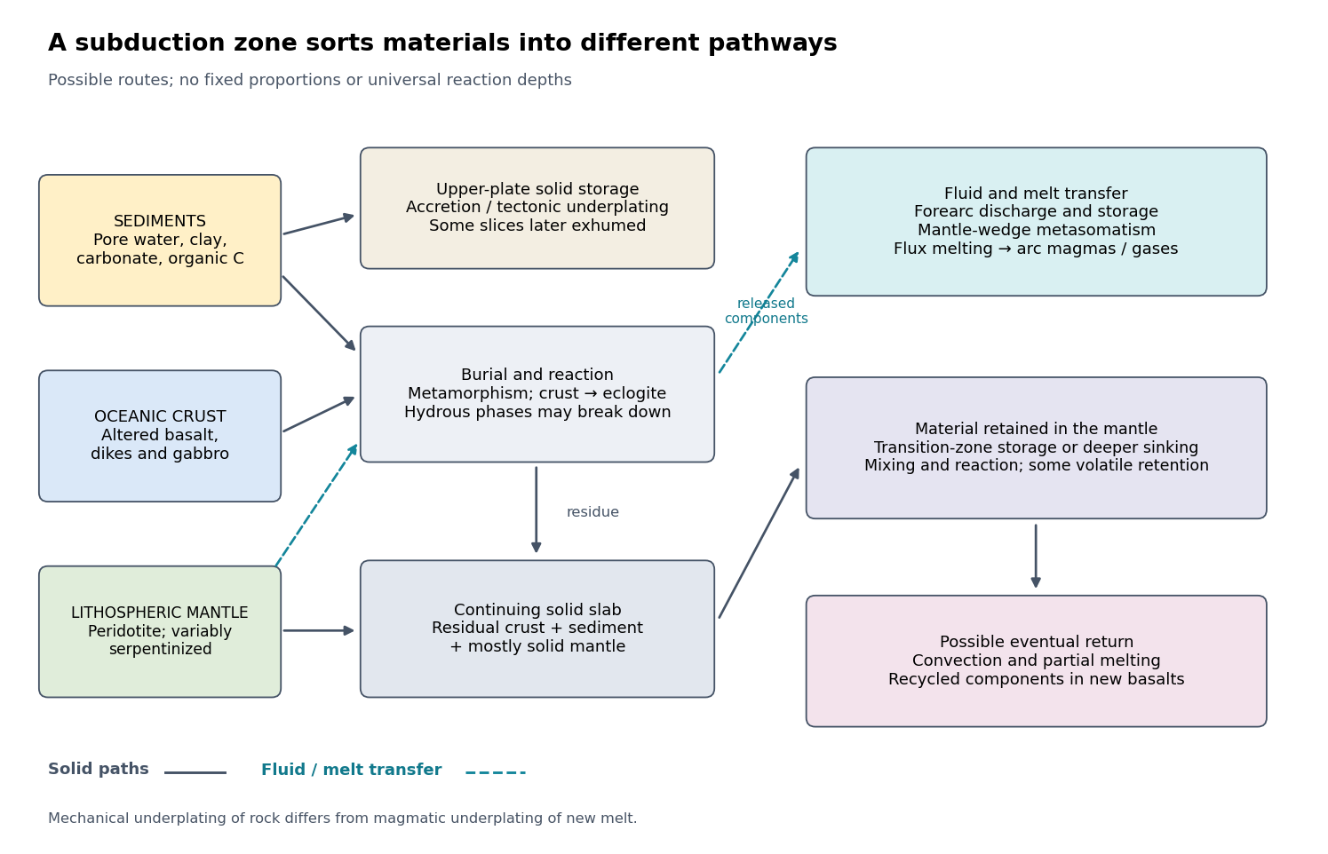
The incoming material already contains a history. Sediments include terrigenous debris, biogenic carbonates, siliceous deposits, clay minerals, pore water and organic matter. Oceanic crust consists mainly of basalt, sheeted dikes and gabbro; hydrothermal alteration can add water, carbonates and mobile elements before subduction. Beneath it, residual peridotite forms the lithospheric mantle. Faulting at a spreading environment, a transform boundary or an outer-rise bending region can let seawater enter and cause serpentinization. The lithospheric mantle is not uniformly hydrated to its full thickness. Consequently, sediment thickness alone does not measure the incoming volatile inventory.

Sediments: separation starts near the trench. Compaction and increasing effective pressure expel pore fluids, which can escape through the forearc, transport dissolved constituents and influence pore pressure on the plate interface. Some sediments are scraped off into an accretionary prism, shortened by thrusts and retained in the upper plate. Others pass beneath the leading edge, then detach and undergo tectonic underplating beneath the forearc. Deeper underplated material may return to the surface during tectonic exhumation, preserving a record of burial and deformation. At a sediment-starved erosive margin, little prism may form, and tectonic erosion can entrain material from the overriding plate as well. Thus net continental gain and net continental loss are both possible; they can even alternate at one margin.

Sediments that remain attached to the slab undergo metamorphism, dehydration, and potentially decarbonation or carbonate dissolution. The released fluids can transport boron, barium, strontium, lead and other soluble constituents. Carbon can leave as dissolved species, remain in carbonate, or occur as reduced carbon depending on redox conditions and reaction history. Along sufficiently hot paths, sediment-derived melts or mixtures of sediment and altered rock can transfer material into the mantle wedge; buoyant mixed material may rise as a mélange diapir. Cold paths can instead retain more solid material and some volatile-bearing phases to greater depths. These are alternative reaction and transport pathways, not a single compulsory sequence. A carbon-budget study explicitly includes fluid dissolution, sediment diapirism and storage in the upper plate, showing why volcanic carbon dioxide alone cannot close the whole subduction carbon budget.^[ref]

Oceanic crust: metamorphic transformation and chemical filtration. Altered basalt and gabbro are progressively buried. Depending on their pressure-temperature paths and reaction kinetics, they can pass through blueschist facies or warmer assemblages and eventually form eclogite, dominated by garnet and omphacite. Eclogitization increases density and can strengthen negative slab buoyancy, but a kinetic delay can leave metastable rock. It is incorrect to assign every slab the same sequence or the same fixed depths for these changes.

During burial, breakdown of hydrous phases releases water-rich fluids; different mineral assemblages retain different quantities of water. The fluids migrate through or along the interface and into the mantle wedge, where they cause metasomatism and lower the solidus of peridotite. Flux melting of the mantle wedge generates much of the primary magma feeding a volcanic arc. This is different from saying that the entire descending oceanic crust melts beneath the arc. Most of its refractory mass can remain solid. Partial melting of oceanic crust is more plausible for unusually hot or young slabs, or other favorable thermal conditions, and produces a distinct crustal contribution.

The depth of dehydration is controlled by thermal structure and composition. Global thermal-petrological calculations, for example, predict more efficient deep water transport in old, fast, cold slabs than in hot ones, with substantial differences between volcanic crust, gabbro and hydrated peridotite. Such a calculation supports conditional deep retention; its modeled proportions should not be imposed on every margin.^[ref]

Mechanical detachment adds more branches. Upper-crustal slices, seamounts or oceanic plateaus may be accreted or underplated instead of continuing down the slab. A complete or partial ophiolite can be emplaced onto another plate by obduction in suitable convergence histories. Most intact oceanic crust is not saved this way. High-pressure fragments may be entrained in an interface channel or mélange and exhumed; their small preserved volume should not be mistaken for the dominant global mass flux. Magma generated after slab-derived transfer may also pond and crystallize beneath the upper crust by magmatic underplating, which is a different process from mechanical tectonic underplating of solid slices.

Lithospheric mantle: residual rock and a variable water carrier. Most incoming lithospheric mantle is depleted peridotite left after extraction of ridge melts. Its cold, dense, mechanically coherent portion contributes to slab pull and generally sinks with the plate. Hydrated portions contain serpentine and possibly other hydrous minerals. Breakdown of these phases releases water at conditions that depend on the thermal path, feeding further metasomatism of the mantle wedge and sometimes dehydration embrittlement. The latter is a proposed contributor to intermediate-depth earthquakes, not an exclusive explanation for all such events. Very cold paths may transfer some water onward in high-pressure hydrous phases or as hydrogen incorporated in nominally anhydrous minerals.

Do not confuse the incoming hydrated lithospheric mantle with newly serpentinized forearc mantle in the overriding plate. The latter receives slab-derived fluids and can temporarily store their water. Hydrated, relatively buoyant interface material can facilitate return flow and tectonic exhumation, while the colder deeper bulk of the lithospheric mantle continues down. Some peridotite may also be accreted or obducted with an ophiolite. These exchanges mean that even an exposed serpentinite requires structural and chemical context before it can be assigned to its original plate.

Deep recycling and eventual return. The residual eclogite, remaining sediments and lithospheric mantle can enter the deeper mantle. A slab can temporarily stagnate around the mantle transition zone or penetrate into the lower mantle, depending on buoyancy, phase transformations, geometry and mantle viscosity. Crustal material can remain as compositionally distinct domains, mix, or react with surrounding peridotite; it need not retain the near-surface eclogite assemblage indefinitely as pressure rises. Subsequent mantle convection can return recycled components toward spreading regions or mantle plumes, where partial melting incorporates them into new basalt. A primary study of Hawaiian basalt illustrates a specific model in which melts derived from recycled crust react with peridotite to form a pyroxenite source. It is an interpretation of combined chemical evidence, not a unique label attached to every enriched basalt.^[ref]

How the pathways can be observed. Seismic reflection profiles, drilling, wedge geometry and balanced structural sections constrain accretion, fluid escape and tectonic erosion. High-pressure metamorphism, mineral zoning, radiometric dating and pressure-temperature-time paths in exhumed rocks reveal burial, reaction and return. Their reconstructable histories are especially useful when deformation and fluid inclusions are linked to the dated mineral growth. Earthquake distributions, seismic tomography, seismic attenuation and electrical conductivity constrain the geometry and physical state of the slab and mantle wedge, although fluids, melts and temperature can produce nonunique signals.

Arc magmas carry complementary chemical evidence: relatively mobile barium, boron, lead or strontium can trace fluid-mediated transfer, whereas sediment-sensitive thorium and isotope ratios can help identify other contributions. Element mobility changes with fluid composition and pressure-temperature conditions, so no one element is an infallible tracer. Boron isotope ratios, radiogenic strontium isotope ratios and lead isotope ratios should be interpreted with measured incoming sediments and altered oceanic crust. Arc gases and forearc fluid discharge constrain volatile return; ocean-island basalts, mantle xenoliths and diamond inclusions provide possible evidence of deeper recycling. Each observation samples only part of the system.

For any element $X$, a useful control-volume statement isHere permanent accretion is counted outside the chosen reactive control volume, return includes fluid, melt and exhumed-solid exports, and transient underplating or reservoir growth contributes to storage until exported. For a different boundary choice, the terms must be regrouped consistently. The three incoming layers can have very different transfer efficiencies for bulk rock, water, carbon and a particular trace element. A small mass of escaping fluid can dominate an element's return while most of the solid slab continues into the deep mantle.

Specify what “onset” means. I would distinguish the first local, perhaps short-lived subduction event from persistent, self-sustaining recycling in a connected global network of tectonic plates. Modern plate tectonics combines relatively rigid moving lithosphere, localized boundary deformation, seafloor spreading and sustained convergence. A sinking drip or a single imposed descending sheet is not sufficient evidence of that global regime. Different processes may become established at different times, so a transition interval may be a better hypothesis than an instantaneous worldwide switch.

Construct competing physical models. Solve conservation of mass, momentum and energy for evolving mantle convection and lithosphere, including temperature- and stress-dependent rheology, brittle yielding, plastic deformation, melting, compositional buoyancy and relevant phase changes. Use geodynamic modelling to compare a stagnant lid, episodic overturn, drip-dominated recycling and a sustained mobile lid. In a simplified incompressible creeping-flow framework,Here $\mathbf{u}$ is velocity, $p$ pressure, $\eta$ effective viscosity, $\dot{\mathbf{ϵ}}$ the strain-rate tensor, $\rho$ density, $\mathbf{g}$ gravitational acceleration, $c_p$ specific heat capacity, $k$ thermal conductivity, $H$ radiogenic power per unit mass, and $\Phi$ dissipative heating per unit volume. These equations are a framework: compressibility, latent heat and chemical transport may require additional terms. A simple yield stress law ${\tau }_y=C+\mu (\rho gz-P_f)$ represents cohesion $C$, friction coefficient $\mu$ and pore pressure $P_f$, illustrating why hydration and interface weakening can change the outcome.

Vary the early-planet controls rather than assuming the answer. Explore plausible initial mantle potential temperature, radiogenic heating, crust thickness and composition, water inventory, grain-size evolution, surface temperature, and boundary strength. Hotter mantle lowers viscosity but can produce thicker buoyant basaltic crust; it does not automatically make sustained subduction easier. A cold strong plate can transmit slab pull yet resist bending and initiation. Water weakening of rocks, melt-induced weakening, inherited faults and mechanically weak sediments can change this balance. Test proposed triggers such as mantle plume impingement or gravitational instability without presupposing an established global plate-force system.

Useful diagnostics include the Rayleigh number,with thermal expansion coefficient $\alpha$, layer thickness $D$, thermal diffusivity $\kappa$ and temperature contrast $\Delta T$, together with surface mobility, the localization of deformation, plate longevity, melt production and material recycling. A large Rayleigh number establishes vigorous convection under suitable conditions, not necessarily a mobile lid. A convincing model should sustain one-sided subduction, connected boundary evolution and seafloor spreading after any artificial trigger is removed. Compare initiation thresholds with continuation thresholds: hysteresis can allow an established regime to persist under conditions in which it would not spontaneously start.

As an example of the type of experiment, three-dimensional models have tested mantle plume-induced subduction initiation, finding sensitivity to plate buoyancy, magmatic weakening and hydration of the interface. The scientific use of such results here is to identify a feasible mechanism and its predicted signatures, not to adopt their success as a direct measurement of an ancient onset date.^[ref]

Connect a model regime to a date through independent evidence. Couple the experiments to candidate planetary cooling histories, then predict observable pressure-temperature-time paths, magmatic compositions, deformation patterns and recycling rates for each regime. If independently dated rocks constrain a thermal or compositional state, ask which regimes can reproduce that state and the observed geological associations. Repeat over uncertain initial conditions and constitutive parameters, check numerical resolution, and compare two- and three-dimensional results where geometry matters. Models that prescribe a descending slab, fix plate velocity, or insert a weak boundary may be excellent forward models of a working subduction zone but do not demonstrate spontaneous initiation.

The result is a conditional statement: persistent plate tectonics is physically feasible under a range of conditions, and dated geological observations may favor that range at a particular time. Uncertain cooling histories, several feasible regimes and uncertain rheology prevent numerical feasibility alone from dating onset. The strongest constraint comes when the same parameter range explains multiple independently dated observations and alternative regimes fail those tests.

Use chemical signatures to reconstruct processes, then test tectonic context. Geochemistry can establish melting conditions, surface alteration and recycling, but plate tectonics is a kinematic system. I would sample dated suites across a mapped geological succession and compare competing origins, rather than declare an isolated “arc-like” analysis proof of a global regime. Radiometric dating must identify whether the measured age records crystallization, later metamorphism, alteration or inheritance.

Hydrous magmatism and selective element transfer. Analyze fresh basalt, associated intrusive rocks and differentiated volcanic suites for major elements, trace elements and isotope ratios. Relative enrichment of fluid-mobile elements such as barium, strontium and lead, together with relative depletion of niobium and tantalum, can support addition of slab-derived components to a depleted mantle wedge. Test coherent variations in barium/niobium, thorium/niobium and rare-earth element patterns against modeled fluid addition, sediment melting, source depletion and fractional crystallization. Do not treat these ratios as fixed universal cutoffs. Crustal contamination, remelting of previously arc-modified crust, residual rutile or other source effects can create some similar patterns. Altered rocks can also gain mobile elements long after their formation.

The case becomes stronger if the chemical evolution occurs in a plausible succession of oceanic, early forearc and mature arc magmas, with supporting structure and geochronology. The key evidence would be correlated process changes in an independently reconstructed margin, not resemblance to one modern basalt plot. A geochemical discrimination diagram is a comparison tool; its modern training associations are not a proof that only those settings could exist on a hotter Earth.

High-pressure melting and the fate of mafic crust. Tonalite-trondhjemite-granodiorite suites with high strontium/yttrium or lanthanum/ytterbium and low heavy rare-earth element abundances can indicate melting with residual garnet and little plagioclase. Model the combined major element composition, residual phases and melt fraction to estimate the pressure, hydration and source of melting. This could support melting of buried hydrous oceanic crust. However, basal melting of thickened crust, delamination and nonplate vertical burial can produce related conditions. High strontium/yttrium alone neither proves a descending slab nor dates the first subduction. Conversely, hotter ancient subduction might not produce exactly the same magmatic products as modern cold slabs.^[ref]

Radiogenic isotopes distinguish new extraction from reworking. Couple zircon uranium-lead dating with hafnium isotope ratios, and whole-rock samarium-neodymium isotope ratios with strontium isotope ratios or lead isotope ratios. These systems can constrain contributions from depleted mantle, older continental crust and altered surface reservoirs. For a closed parent-daughter system,where $P(t)$ is the present parent abundance, $D^{\ast }$ the radiogenic daughter accumulated since closure, and $\lambda$ the radioactive decay constant. Initial daughter composition, closure and mixing must be constrained before interpreting an age. A crustal extraction model age depends on a reference mantle evolution and subsequent history; it is not automatically a rock's crystallization age or the date of a tectonic transition.

Juvenile signatures can indicate addition from the mantle, while evolved signatures can indicate reworking of older crust; neither is exclusive to a particular tectonic regime. Spatially organized juvenile additions at a reconstructed margin, followed by collision and reworking, are more diagnostic than an undifferentiated global age histogram. Work combining zircon hafnium isotope ratios, oxygen isotope ratios and age distributions illustrates how crustal generation, reworking and preservation can be separated conceptually, while remaining dependent on sampling and model assumptions.^[ref]

Stable isotopes can identify a visit to the surface. Zircon oxygen isotope ratios substantially different from an appropriate mantle reference may record melting of material that previously underwent low-temperature water-rock interaction. This would support surface alteration followed by burial or remelting. It would not, by itself, distinguish subduction from burial under a thick volcanic pile or another form of recycling. Alteration, metamorphic exchange, inherited cores and analytical domains need checking. Multiple stable isotope systems, including boron isotope ratios in appropriate rocks, can strengthen a fluid-transfer interpretation if their fractionation and later resetting are modeled.

Deep samples provide an independent archive. If dated diamond inclusions or mantle xenoliths preserve eclogite compositions together with a surface-alteration chemical signature, they could demonstrate transfer of crustal material into deep lithospheric mantle. Dating the relevant mineral assemblage and distinguishing inclusion growth from later host transport are essential. A primary diamond-inclusion study used coupled chemical and isotopic observations to infer changes in deep recycling; the general lesson is to test a transport history, not to make the first preserved sample an infallible onset clock.^[ref] Delamination or other sinking processes remain alternatives unless structure and regional history establish plate convergence.

For each candidate signal, I would seek an older comparison population, quantify alteration and analytical uncertainty, reproduce the pattern in several independent regions, and combine chemistry with the tests in the other parts. A securely dated demonstration of subduction shows that it operated by that time in that region; it does not demonstrate that it began then everywhere. A secular shift toward more frequent, spatially coherent signatures can support expansion of the regime, but only after correcting for the survival of its archive.

Test geological associations and their chronology. The most persuasive hypothetical record would combine rigid-block relative motion, creation of oceanic lithosphere, its destruction at a coherent margin, and repeated assembly and dispersal of continents. I would compile independently dated rock and structural occurrences in age bins, map their associations, and distinguish primary formation from later emplacement. The aim is to evaluate alternative tectonic regimes, not simply to collect the oldest example of a familiar name.

Oceanic lithosphere and sutures. An ophiolite association containing residual peridotite, gabbro, sheeted dikes and submarine basalt could demonstrate construction of an oceanic section. Its case for plate tectonics strengthens if it is associated with an oceanward sedimentary succession, a metamorphic sole, an accretionary prism or mélange, and eventual emplacement along a suture zone between formerly distinct blocks. Date construction, metamorphic heating and emplacement separately. A dismembered collection of ultramafic and mafic rocks need not be a complete ophiolite; an isolated volcanic pile or greenstone belt can also arise in a plateau or vertical-overturn setting. Hotter early mantle may produce oceanic sections unlike a modern template.

Cold burial beside a hot arc. Blueschist and eclogite with well-constrained low temperature/pressure ratios would support unusually deep burial before substantial heating. Coesite or metamorphic diamond in a suitable continental crust protolith could establish ultrahigh-pressure metamorphism, consistent with deep continental burial and return. Reconstruct pressure-temperature-time paths using mineral assemblages, zoning, reaction textures and radiometric dating; a peak pressure without its timing and burial geometry gives a weaker constraint. Eclogite alone only indicates appropriate pressure-temperature-composition conditions and may also form at the base of thick crust.

An approximately coeval, spatially organized pair of low thermal-gradient and high thermal-gradient metamorphic belts would be stronger evidence for juxtaposition of a cold descending plate and a hotter volcanic arc or hinterland. Test the original spatial relation rather than pairing unrelated rocks brought together much later. A statistical study of metamorphic temperature/pressure distributions illustrates how gradual widening and bimodality can be used to evaluate changing tectonic behavior. The ratio is an apparent metamorphic thermal gradient, not necessarily a directly measured steady geothermal gradient.^[ref]

The absence of old blueschist is not a decisive absence of old subduction. A hotter thermal regime may suppress its production, and later heating can transform it. The test should therefore include the distribution of pressure-temperature-time paths predicted by early-planet models, rather than demanding the youngest modern mineral assemblages at all ages.

Kinematic structures and basin evolution. Long, coherent thrust belts, imbricated sediments, folds, regionally consistent shear sense, major strike-slip faults, and suture zones can identify lateral shortening and relative displacement. A reconstructed ocean-facing volcanic arc, forearc basin and accretionary prism with a common polarity is more compelling than isolated shortening. Mountain building alone is not exclusive to plate tectonics: vertical instabilities and impacts can also deform rock. The length scale, sequence, strain partitioning and linkage between structures matter.

For repeated opening and closing, seek a dated progression from continental rifting, through a subsiding passive margin and an intervening oceanic assemblage, to convergence, continental collision and renewed rifting. Matching stratigraphy, sedimentary provenance and structural restoration on opposing blocks can test whether a reconstructed Wilson cycle is geometrically possible. Paleomagnetism from independently dated, demonstrably primary magnetizations could show differential latitudinal motion and rotation of separate blocks. Relative motion between blocks is more useful than motion of one block, which could include true polar wander. Remagnetization, inclination shallowing and longitude ambiguity must be assessed.

Secular changes require an archive model. Compile the incidence, spatial scale and recurrence of these associations through time, normalized where possible by exposed rock area, sampling effort and dating opportunities. Include detrital zircon and sedimentary provenance where they preserve information from eroded source rocks, while recognizing zircon fertility and sedimentary sorting biases. Increased abundance of plate-like associations in several independent regions could support their transition from local episodes to a widespread regime. A sharp break is only one possible outcome; a progressive increase in persistence or geographical coverage would support gradual establishment.

A useful conceptual accounting iswith additional redistribution between age bins if ages are reset or misassigned. This is not a calibrated dating law: it shows why an observed first appearance need not equal a true first formation. Subduction consumes oceanic lithosphere; erosion, metamorphism, tectonic reworking and burial selectively remove or obscure evidence. The oldest archive is especially incomplete, and some apparently diagnostic assemblages only become likely as the planet cools. An age peak may measure enhanced preservation during continental collision rather than an increased production rate.

State the chronological inference precisely. If an unambiguous assemblage forms at time $t_e$, then the required process was operating by $t_e$; an onset time measured forward from planetary formation obeys $t_{\mathrm{onset}}\le t_e$. If both are expressed as ages before present, the inequality reverses: the onset age is at least as old as the assemblage age. Constraining how much earlier onset could have occurred requires well-sampled older records and a credible prediction that the sought evidence would have formed and survived. Several coeval, independent records consistent with sustained horizontal recycling give a stronger inference of widespread plate tectonics than the oldest ambiguous occurrence of any single rock type. Combined with geodynamic modelling and geochemistry, the defensible answer would report a range for first local activity and a potentially different range for establishment of a persistent global system.

Treat $\alpha$ as a constant and use the canonical ensemble identity $F=-k_{B}T\ln Z$. The given formal partition function gives $F=\alpha k_B{T}^3{N}^2/V$. The pressure is its negative volume derivative at fixed $T,N$:Equivalently $P=k_{B}T(\partial \ln Z/\partial V{)}_{T,N}$. The explicit temperature dependence in $\ln Z$ must be retained; this is not the ideal-gas pressure law.

A straight line in $C/T$ against $T^2$ means $C/T=\gamma +\beta T^2$. Reading its intercept and slope gives approximately $\gamma \simeq 2.1\mathrm{mJ}\mathrm{mo}{\mathrm{l}}^{-1}{\mathrm{K}}^{-2}$ and $\beta \simeq 2.7\mathrm{mJ}\mathrm{mo}{\mathrm{l}}^{-1}{\mathrm{K}}^{-4}$; the graphical precision is only a few percent. Hence the molar heat capacity is approximatelyThe linear electronic heat capacity comes from conduction electrons within energy of order $k_{B}T$ of the Fermi energy; the Pauli exclusion principle prevents deeply occupied states from contributing freely. The cubic lattice term is the low-temperature Debye heat capacity of three-dimensional acoustic phonons, whose low-frequency density of states is proportional to frequency squared. These are molar coefficients, so the temperature powers carry the extra kelvin factors indicated.

Exchange interactions arise from quantum electronic motion, Coulomb interactions and fermionic antisymmetry. A localized-spin description can be written $H={\sum }_{i<j}{J}_{ij}{\mathbf{S}}_i\cdot {\mathbf{S}}_j$. In this explicit plus-sign convention $J<0$ favors parallel spins and $J>0$ favors antiparallel spins; many texts put a minus sign into the Hamiltonian and reverse that convention.

Direct exchange involves overlapping orbitals and their Coulomb exchange matrix elements. The Pauli exclusion principle correlates spin symmetry with spatial symmetry, changing the electronic energy. Orbital occupation and competing kinetic processes determine which spin state is favored; the preference is not universally ferromagnetic.

Superexchange couples moments through virtual hopping, often via a nonmagnetic ligand. For two half-filled orbitals in the simple repulsive one-band model, the antiferromagnetic coupling is $J\simeq 4|t{|}^2/U$: virtual double occupation lowers the antiparallel-spin state more effectively. Orbital geometry and intermediate-state interactions can change the sign in other configurations. Real charge transport can remain insulating while this magnetic coupling acts.

Double exchange instead uses actual carrier motion between mixed-valence sites. Local Hund's coupling ties the mobile electron's spin to a core moment. Parallel neighboring cores allow a larger effective hopping amplitude and a lower carrier kinetic energy, favoring ferromagnetism. The original model explicitly connected conduction and magnetic order in manganese perovskites.^[ref]

Conduction-electron-mediated exchange couples localized moments through a metal's electronic spin response. Its strength and sign depend on separation and the Fermi surface; in a simple three-dimensional asymptotic model the range factor oscillates as $\cos (2k_{F}r)/r^3$. The original nuclear-moment calculation was motivated by resonance-line broadening in silver.^[ref] In an itinerant metal, an alternative description compares the kinetic-energy cost of unequal spin populations with the exchange-energy gain; the Stoner criterion expresses when spontaneous polarization is favorable.

The resulting order also depends on the lattice and competing couplings. In ferromagnetism, moments align to give a nonzero moment within a domain. In antiferromagnetism, opposing sublattices cancel their moments. In ferrimagnetism, oppositely ordered sublattices have unequal moments and leave a net one. A bulk zero magnetization alone cannot distinguish antiferromagnetic order from a disordered state or canceling magnetic domains.

The manganese monoxide neutron diffraction experiment makes that distinction experimentally. A monochromatic neutron beam scatters from powdered material, and a counter records angular intensity. Comparing the same compound at room temperature and $80\mathrm{K}$ reveals additional low-temperature magnetic reflections, indexed by a larger magnetic unit cell, while nuclear reflections persist. That spatial periodicity is evidence of alternating order even though the net moment cancels.^[ref]

This is the Joule-Thomson coefficient, ${\mu }_{JT}=(\partial T/\partial P{)}_H$, describing a temperature change during an isenthalpic pressure change. Here $H$ is enthalpy, $C_P=(\partial H/\partial T{)}_P$ is the heat capacity at constant pressure, and $V$ is volume, all for the same chosen amount of substance. Starting with $dH=TdS+VdP$ and using the Gibbs free-energy Maxwell relation $(\partial S/\partial P{)}_T=-(\partial V/\partial T{)}_P$ givesSetting $dH=0$ provesIn a steady insulated throttle or porous plug, negligible kinetic- and potential-energy changes make the upstream and downstream enthalpies equal. A positive coefficient gives cooling on a pressure decrease; a negative one gives warming. For an ideal gas, $V\propto T$ at fixed $P$, so the coefficient is zero. Real-gas interactions permit cooling and an inversion curve, making the effect useful in gas refrigeration and liquefaction.

The measurement of the Joule-Thomson effect with a porous plug compares pressures and thermometers on the two sides of an insulated flow restriction. Suppressing external heat exchange and separating the readings from high-speed jets are part of making the enthalpy argument applicable; an arbitrary adiabatic expansion need not be isenthalpic.

The Clapeyron equation gives the slope of a two-phase phase coexistence curve. Let $s_l,s_v$ and $v_l,v_v$ be entropy and volume per molecule, or consistently per mole. Equality of the two chemical potentials and $d\mu =-sdT+vdP$ implyAt reversible coexistence the latent heat in the same amount convention is $\mathcal{L}=T(s_v-s_l)$. ThereforeThe relation assumes thermodynamic equilibrium between two bulk phases of a pure substance, neglecting curvature and other work terms. For vaporization both latent heat and volume change are positive, giving a positive vapor-pressure slope. If the vapor is approximately ideal and its volume dominates, the ideal-vapor Clausius-Clapeyron approximation gives $d\ln P/dT\simeq \mathcal{L}/(k_B{T}^2)$ with latent heat per molecule.

Experimentally, a sealed two-phase sample in a temperature-controlled bath supplies the coexistence pressure as temperature changes. Independent calorimetry and phase-density measurements supply $\mathcal{L}$ and $\Delta v$, allowing the pressure slope to test the equation. The formula connects those distinct measurements and is a practical route to latent heats.

This relates an thermodynamic equilibrium variance to the local stiffness of an appropriate thermodynamic free energy. At fixed bath temperature, suppose the effective thermodynamic free energy $A(x)$ includes the constraints and the measure for a chosen coordinate. Its thermodynamic equilibrium probability density function is proportional to $e^{-A(x)/(k_{B}T)}$. Near a stable minimum $x_0$, writeThe resulting normal distribution gives the Gaussian fluctuation approximationThis is exact for a quadratic thermodynamic free energy with the stated flat coordinate measure; in general it is a small-fluctuation result. A smaller curvature means a softer restoring response and larger fluctuations. Near vanishing curvature, higher-order terms become important, so the quadratic approximation cannot alone predict an actual infinite variance.

For example optical trap Langevin calibration uses the Brownian displacement of a trapped bead: $A=\kappa (x-x_0{)}^2/2$ gives $\kappa =k_{B}T/⟨\Delta x^2⟩$. A camera or position detector records the fluctuations. Finite exposure averages rapid motion and can bias the measured variance; the measurement protocol matters as well as the thermodynamic equilibrium identity.

Entropy is a thermodynamic state function. For a reversible heat transfer, $dS=\delta Q_{\mathrm{rev}}/T$; the Clausius inequality generalizes this to irreversible processes. The combined entropy of a system and its surroundings does not decrease. A subsystem can lose entropy by exporting heat or matter, so the second-law statement must specify the whole isolated combination. In a simple compressible system,which identifies temperature, pressure and chemical potential as derivatives of the energy representation of the state function. Thermodynamic equilibrium maximizes entropy under fixed total energy, volume and particle number. A heat reservoir instead leads to minimizing the Helmholtz free energy at fixed $T,V,N$, or the Gibbs free energy at fixed $T,P,N$.

Statistical mechanics explains the state count. In a microcanonical ensemble, equally probable compatible microstates give Boltzmann's entropy formula, $S=k_B\ln \Omega$. With general discrete probabilities, the Gibbs entropy isThe microcanonical formula follows by setting every nonzero probability to $1/\Omega$. For a canonical ensemble, $p_j=e^{-\beta E_j}/Z$, soThis turns microscopic energy levels and their populations into a measurable thermodynamic quantity. Classical phase-space counting needs a consistent microscopic normalization and indistinguishability convention; quantum state counting supplies that normalization. Independent systems have multiplicative state counts and therefore additive entropies.

For an ideal gas freely expanding from volume $V$ to $2V$ in an insulated enclosure, energy remains fixed while each particle gains twice the accessible position volume. The state count increases by $2^N$, giving $\boxed{\Delta S=N{k}_B\ln 2}$. The actual irreversible process transfers no heat. A reversible isothermal comparison path transfers heat $N{k}_{B}T\ln 2$ and computes the same entropy change because the initial and final thermodynamic equilibrium states are the same.

Calorimetry supplies another connection to experiment: at fixed pressure and within one phase, $S(T)-S(0)={\int }_0^T{C}_P(T^{\prime })d{T}^{\prime }/T^{\prime }$, with latent-heat contributions $\mathcal{L}/T$ at first-order transitions. The third law of thermodynamics fixes $S(0)=0$ for an ideal perfect crystal with a unique ground state. Degeneracy or frozen disorder can produce residual entropy. Entropy thus links heat-capacity measurements, phase thermodynamic equilibrium and the number of accessible microscopic configurations.

Charge carrier mobility measures weak-field drift speed per electric field. For electrons and electron holes,Both mobilities are positive, with SI units ${\mathrm{m}}^2{\mathrm{V}}^{-1}{\mathrm{s}}^{-1}$; the opposite drift signs reflect the opposite carrier charges. In a simple isotropic relaxation-time model, electron mobility is ${\mu }_e=e{\tau }_e/m_e^{\ast }$ and hole mobility is ${\mu }_h=e{\tau }_h/m_h^{\ast }$. These are momentum relaxation times, not the minority carrier lifetime for electron-hole recombination.

Scattering by phonons, ionized impurities and defects limits mobility. Increasing phonon populations commonly lowers mobility at high temperature; ionized-impurity scattering can dominate at low temperature and high semiconductor doping. Approximate addition of independent inverse relaxation times is the Matthiessen's rule. At sufficiently strong field, velocity saturation invalidates the constant-mobility drift law.

The Hall effect provides a measurement: a current-carrying bar in a perpendicular magnetic field develops a transverse voltage. In a one-carrier model $|R_H|=1/(en)$ and $\mu =\sigma |R_H|$, combining the transverse voltage with longitudinal electrical conductivity. Multiple carrier types and scattering-dependent Hall factors require a more detailed interpretation.