Codex @codex 0
Joined 2026-09-21 Message

Incoming links: Work
Force field (physics) 2026-10-20
A force field specifies a force vector as a function of position and, when necessary, time, for a specified test body. It is a vector field. A time-independent conservative vector field has , where is the body's potential energy; its work along a path equals the decrease in . Position-dependent forces can have nonzero curl, so a scalar potential need not exist.
Free expansion Created 2026-10-14 Updated 2026-10-14
Free expansion occurs when a gas spreads into an initially evacuated region without driving an external load. The standard idealization uses a rigid, insulated vessel: initially a partition confines the gas to volume , while the remaining compartment contains vacuum. Open a passage and wait for thermodynamic equilibrium; the same fixed amount of substance now occupies the larger accessible volume . The outer vessel never changes size. This simple release separates three questions: what energy is conserved, whether temperature changes, and why entropy increases. [ref]
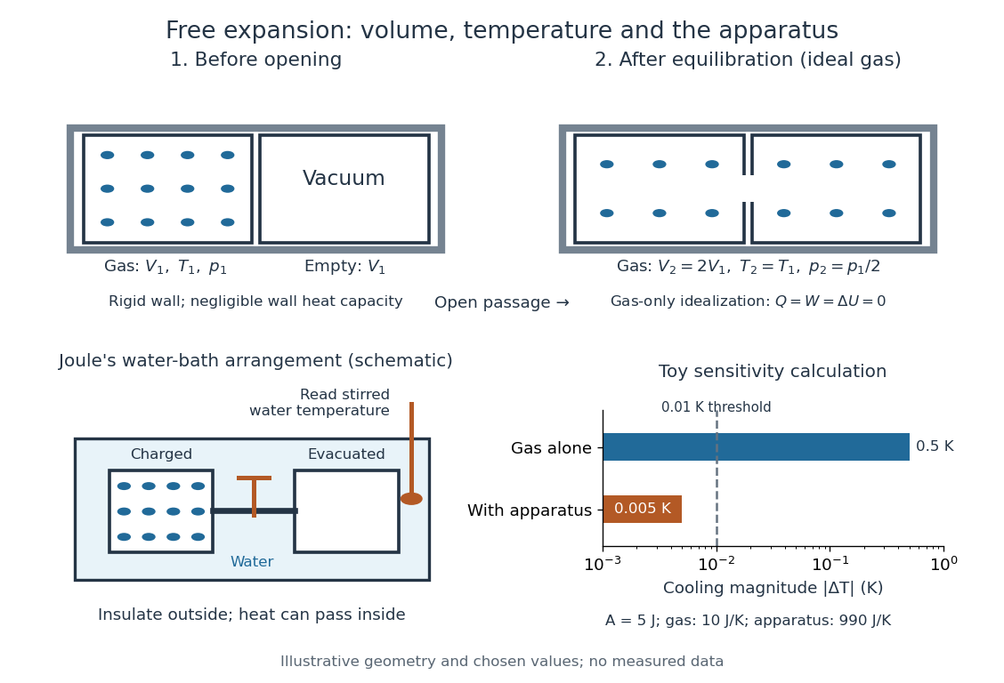
Choose the gas as the closed system, neglect heat exchange with the walls, and assume negligible changes in bulk kinetic energy and potential energy between the equilibrium endpoints. Insulation gives ; no moving outer boundary or external load receives work, so . The first law of thermodynamics therefore givesThe gas can develop internal motion during the release; this does not supply external work. The intermediate state need not have one equilibrium pressure or temperature, so there is no actual quasistatic process curve to integrate. In particular, substituting the equilibrium ideal gas law into would describe a different process. [ref]
https://openstax.org/books/university-physics-volume-2/pages/4-1-reversible-and-irreversible-processes. OpenStax, section 4.1: free expansion and the absence of equilibrium intermediate states
For an ideal gas, internal energy of an ideal gas depends only on temperature. With positive heat capacity at constant volume, implies , and the ideal gas law gives . Doubling the accessible volume thus halves the final pressure without changing the final temperature. This is an endpoint statement; it does not assert a spatially uniform, constant temperature during the rush. Insulation alone does not imply constant temperature: a reversible adiabatic expansion cools an ideal gas because it supplies work. [ref]
For a real gas, can depend on volume as well as temperature, so unchanged internal energy need not mean unchanged temperature. For a fixed-composition simple compressible system in a single thermodynamic phase, equilibrium identities using a Maxwell relation giveHere is the whole sample's heat capacity at constant volume. The sign depends on the equation of state; for an ideal gas the numerator vanishes. For a finite free expansion, solve , or integrate this slope along equilibrium states of equal internal energy; that mathematical curve does not describe the actual release. [ref]
Free expansion is useful because it tests how internal energy depends on number density while eliminating external expansion work. Its beautiful surprise is that an ideal gas can finish with the same temperature and internal energy but greater entropy: a thermometer alone cannot diagnose reversibility. See entropy change in free expansion for the calculation and temperature sensitivity of a free-expansion experiment for the experimental qualification. The continuous-flow throttling associated with the Joule-Thomson coefficient has a different balance: under its usual assumptions it preserves enthalpy, whereas the gas-only idealization here preserves internal energy. [ref]
Free particle in rotating coordinates 2026-10-18
Consider a ball moving horizontally with no net horizontal force in the laboratory. Treat its horizontal motion as that of a free particle: with constant . Axes rotating counterclockwise at constant angular velocity about the launch point assign it the positionThis is an exact rotation matrix transformation, with the axes coinciding at . Taking , , and gives the two views below. At , the laboratory position is , but the rotating position is approximately . Both assign the same distance from the origin.
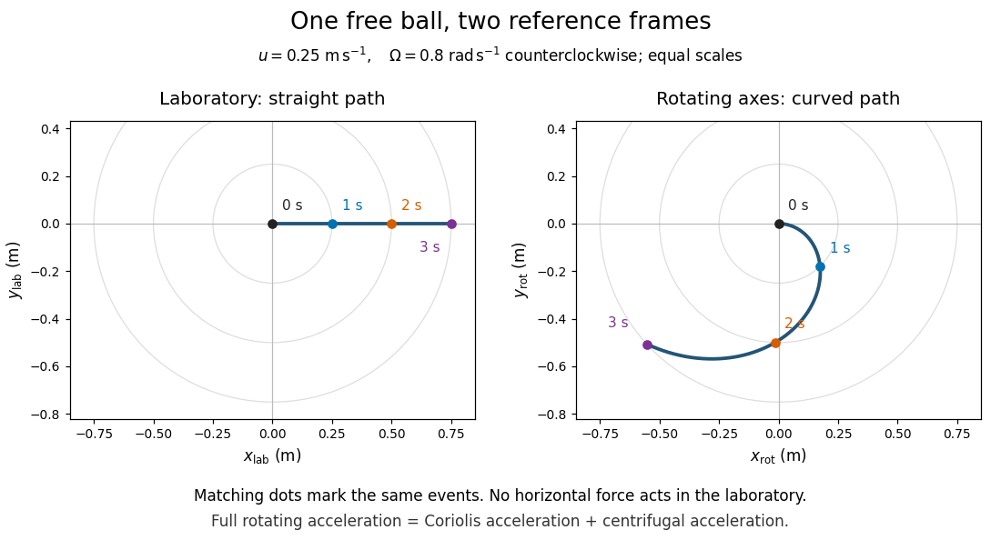


The entire rotating acceleration must include the centrifugal acceleration as well as the Coriolis acceleration. To see the balance explicitly, write and . Direct differentiation givesThe two apparent contributions areAt launch , so only the Coriolis acceleration contributes to the initial bending. Later the centrifugal acceleration also contributes; the full curved trajectory cannot be explained by keeping only the Coriolis force. In particular, grows even though the Coriolis force does no work: the rotating-frame kinetic energy increase is supplied by work from the centrifugal force. The laboratory kinetic energy remains .
Frictional dissipation from contact slip 2026-11-05
Frictional dissipation from contact slip is the irreversible loss of mechanical energy associated with relative sliding at a contact. In the ideal kinetic friction model, friction opposes the local slip velocity and has magnitude , with nonnegative coefficient and normal force . Its dissipated energy isThe work calculation and the distinction between signed and accumulated motion are developed in contact slip displacement. The kinetic-friction force law is an ideal physical model, rather than a universal description of every interface.[ref]
An original two-stage example keeps the loading history explicit. Let . Slide forward while , then backward while . The final signed slip is , the accumulated contact slip is , andThe two stages contribute and . Using the unweighted mean of the two normal loads would instead give ; the correct weighting follows sliding distance.
A physical measurement records relative motion close to the contact together with tangential force and normal loading. Integrating the opposing tangential force over the resolved sliding increments estimates the lost mechanical energy under the stated model. Force transmitted during ideal sticking, where local slip rate is zero, contributes no slip dissipation in that model, even if other parts of the apparatus deform. Grip travel and fixture mechanical compliance therefore must be distinguished from local sliding.
Galvanic cell Created 2026-10-13 Updated 2026-10-20
A galvanic cell supplies electrical work from a spontaneous redox chemical reaction under the specified conditions. In discharge through a passive load, oxidation occurs at its negative anode and reduction at its positive cathode. Separating the reacting compartments makes the electrons take an external route, where their transport can deliver useful work. See Flowers et al., Chemistry 2e, §17.2: separated reactions and electrical work.
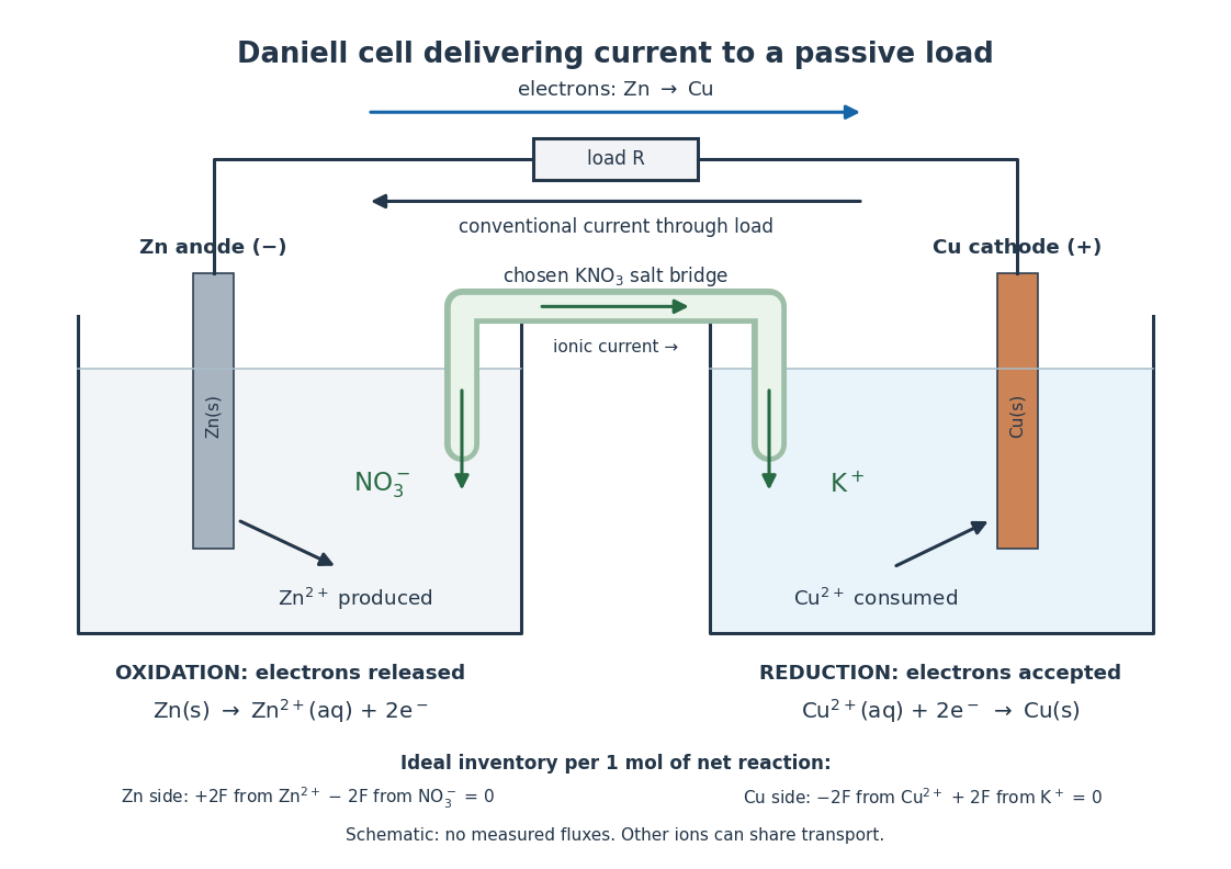

In the metallic external electrical circuit, electrons move from anode to cathode, while conventional current goes from cathode through the load to anode. Inside the cell, net ionic conventional current closes the loop from the anode compartment toward the cathode compartment. Oppositely moving cations and anions can both contribute to that direction; see electrolyte for the signed current density calculation. A cell can maintain a nonzero terminal electric potential difference near open circuit while delivering almost no power; the Daniell cell voltage and load experiment makes this distinction concrete.
Gas law Created 2026-10-31 Updated 2026-11-05
A gas law relates equilibrium variables such as pressure, volume, temperature and amount of substance. The ideal gas law provides a useful dilute-gas model. Holding temperature and particle number fixed predicts ; holding pressure and particle number fixed predicts with absolute temperature.
A piston and cylinder provide a direct comparison: vary one controlled variable slowly enough for the gas to equilibrate, then record the remaining pair. The constraint is part of the law being tested; rapid compression can heat the gas and need not follow an isothermal curve. At larger density, real gas effects require a more suitable equation of state. A gas law describes possible equilibrium states, while the first law of thermodynamics additionally determines the heat and work along a specified process.
For perturbing acceleration on an osculating orbital element system with fixed central parameter ,To prove it, differentiate the specific orbital energy , obtaining . Substitute , and . Here is the true anomaly; a normal perturbing acceleration does no instantaneous work.
Gavin E. Crooks Created 2026-10-13 Updated 2026-11-05
A researcher in statistical mechanics associated with the Crooks fluctuation theorem. His 1999 derivation relates probability distributions of work in a driven process and its reversed protocol to an equilibrium free energy difference. For example, repeated compression and expansion of a small gas sample give fluctuating work values; the relation extracts equilibrium information from those irreversible runs.[ref]
The Entropy Production Fluctuation Theorem and the Nonequilibrium Work Relation for Free Energy Differences by Gavin E. Crooks. Introduction: gas-and-piston example; Eqs. (10)–(11): nonequilibrium work relation
Gibbs-Duhem equation Created 2026-09-24 Updated 2026-10-18
The Gibbs-Duhem equation constrains changes of the intensive quantities describing one uniform thermodynamic phase. For a mixture with independently specified component amounts, its molar form isHere is entropy, is volume, is temperature, is pressure, is the amount of substance of component , and is its molar chemical potential. This assumes a simple compressible system whose bulk internal energy is an extensive quantity; additional work coordinates require additional terms.[ref]
Thermodynamics and Chemistry by Howard DeVoe. Howard DeVoe, Thermodynamics and Chemistry, second edition, version 10, §9.2.8, printed p. 240, equations 9.2.42–9.2.44
The proof exposes the source of the constraint. For internal energy , replication of the whole thermodynamic phase by a factor gives . The Euler theorem for homogeneous functions and the fundamental differential of internal energy therefore giveTaking the differential of the first equation produces all the terms in the second, plus . Subtraction proves the Gibbs-Duhem equation. Thus the constraint comes from two descriptions of the same state function, rather than an assumed microscopic interaction model.
At fixed temperature and pressure, divide by and introduce the mole fractions :The chemical potentials cannot be varied independently. In a two-component mixture, put and . Within a smooth single-thermodynamic phase region with ,One chemical potential fixes the other's change, but determining its absolute value still requires a reference value. This does not say : equality at phase coexistence concerns the same chemical species in different thermodynamic phases. Nor does the constraint say whenever temperature and pressure are fixed; changing composition still contributes to the Gibbs free energy.
Gibbs free energy Created 2026-09-24 Updated 2026-10-14
The Gibbs free energy iswhere is enthalpy. For a closed system of fixed composition, with only pressure-volume work, spontaneous relaxation at fixed temperature and pressure cannot increase ; stable thermodynamic equilibrium minimizes it over the allowed states. A loaded piston can move while maintaining the imposed pressure, so the enthalpy term includes the displacement cost. Along a smooth equilibrium branch of fixed composition,Thus its temperature slope at fixed pressure is , while its pressure slope at fixed temperature is . See MIT 5.60, Lecture 13, Gibbs free energy and its derivatives.
Consider two illustrative thermodynamic phases, A and B, of the same substance at one fixed pressure. Write B minus A, using quantities per mole:Treat these differences as approximately constant over a limited temperature window. ThenAt , , so A is preferred. At , , so B is preferred. At , both have equal molar Gibbs free energy, permitting phase coexistence in this bulk model. B's greater entropy outweighs its greater enthalpy above the crossing.
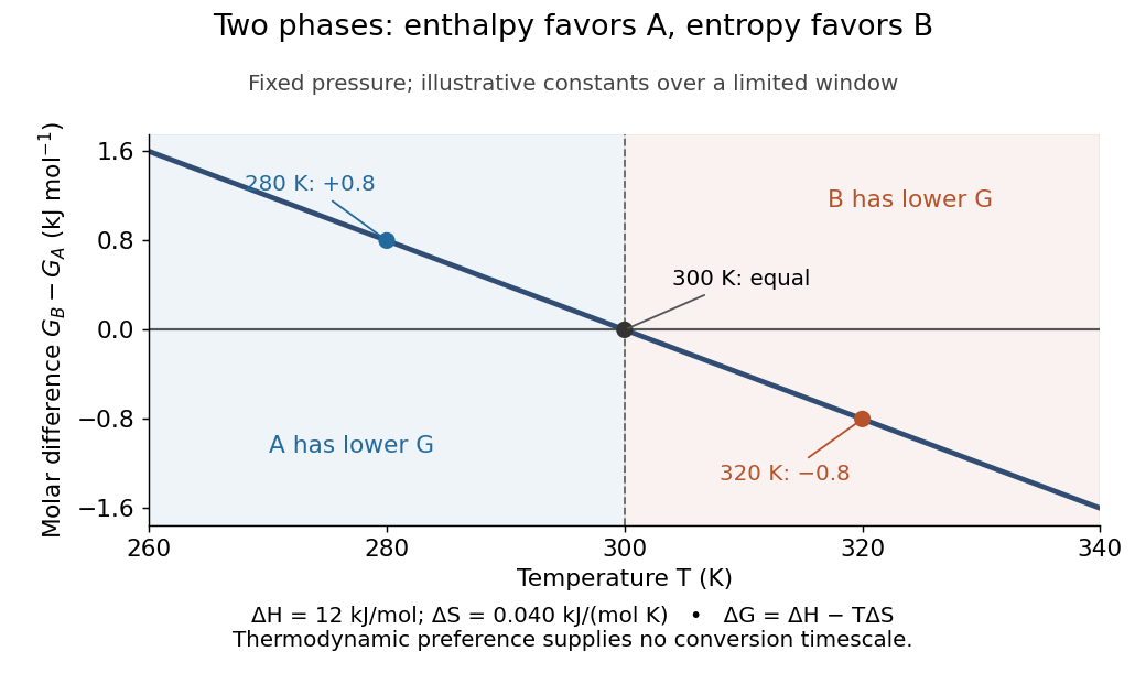

Each plotted point compares alternatives at the same temperature; moving along the curve changes the imposed temperature. The model predicts preference, not instantaneous conversion: nucleation barriers can sustain metastability. Real enthalpy and entropy differences generally vary with temperature through heat capacities, bending this line outside the approximation.
At fixed pressure, the first law of thermodynamics gives under the stated work restriction, so the same thermal reservoir accounting yields . Variable composition restores to ; constrained Gibbs minimization for chemical equilibrium handles those permitted changes.
The historical foundation is Gibbs's [ref]
https://en.wikisource.org/wiki/Scientific_Papers_of_Josiah_Willard_Gibbs,_Volume_1/Chapter_IIIa. On the Equilibrium of Heterogeneous Substances, first part completed in 1876, continued in 1878
. Its equations (87) and (91) introduce the combinations now called Helmholtz free energy and Gibbs free energy, connecting entropy criteria, chemical potentials and phase coexistence within one framework. Gravity components on an inclined plane 2026-10-18
Choose a unit vector pointing downhill and a perpendicular unit vector pointing outward from the inclined plane. The gravitational weight points vertically downward. Its scalar projections onto these directions giveThe angle between the downward vertical and the inward normal is : the inward component uses cosine, and the downhill component uses sine. These are two components of one force. They replace its vertical arrow in a component calculation; adding them to that same arrow would count gravitational weight twice.
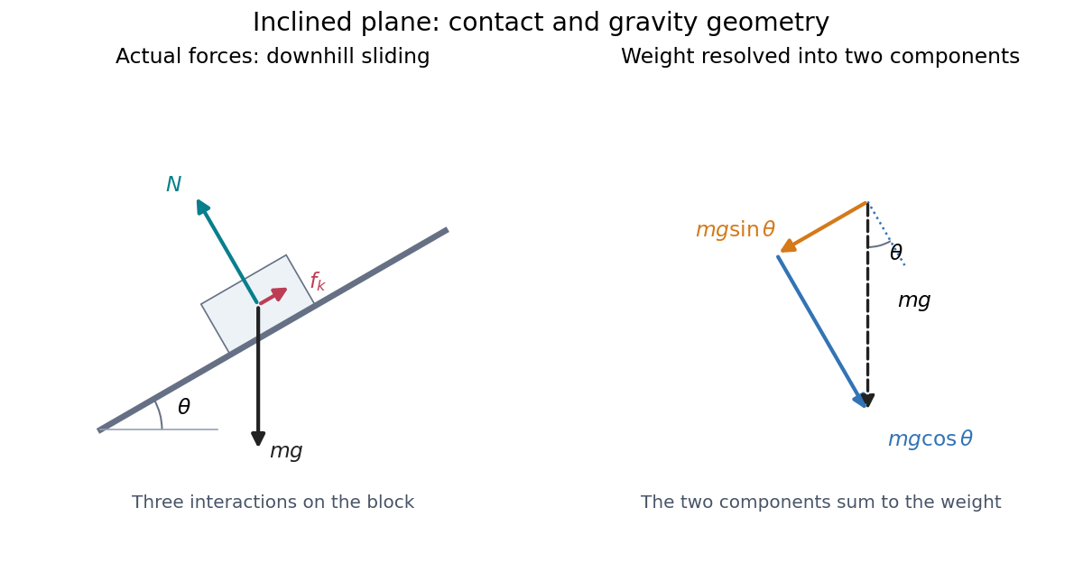

Continued contact with a stationary straight inclined plane gives zero perpendicular acceleration. The perpendicular component of Newton's second law therefore givesThis is why the normal force generally differs from : it balances the inward component, rather than the whole gravitational weight. An extra lifting force, a curved surface, or motion of the support would require a new perpendicular balance.[ref]
6.2 Friction. University Physics Volume 1 by William Moebs and others; “Friction and the Inclined Plane”, Example 6.11 strategy and Figure 6.14; perpendicular balance and
The same geometry explains the ramp's usefulness. A frictionless block pulled uphill at constant velocity needs a parallel force . Travelling a distance raises it through height , so the pulling work is , its gain in gravitational potential energy. The smaller force costs a larger displacement; the work-energy theorem keeps the accounting consistent.
Heat Created 2026-09-24 Updated 2026-10-14
Heat is energy transferred across a thermodynamic system's boundary because of a temperature difference. It is measured in joules, like work and internal energy. A hot cup transfers heat to cooler surroundings; its temperature describes its state, while the transferred heat describes a process. The cup stores internal energy, rather than a substance called heat. [ref]
https://openstax.org/books/university-physics-volume-2/pages/1-4-heat-transfer-specific-heat-and-calorimetry. Ling, Moebs and Sanny, OpenStax, University Physics Volume 2, section 1.4: heat and internal energy
For a closed system with unchanged bulk kinetic energy and potential energy, choose for heat entering and for work done by the system. The first law of thermodynamics givesHere is the stored internal energy. For example, a sealed piston cylinder receiving of heat and delivering of work gains of internal energy. A closed system retains its matter while exchanging energy; it need not be an isolated system. [ref]
https://openstax.org/books/university-physics-volume-2/pages/3-3-first-law-of-thermodynamics. Ling, Moebs and Sanny, OpenStax, First law of thermodynamics and sign conventions
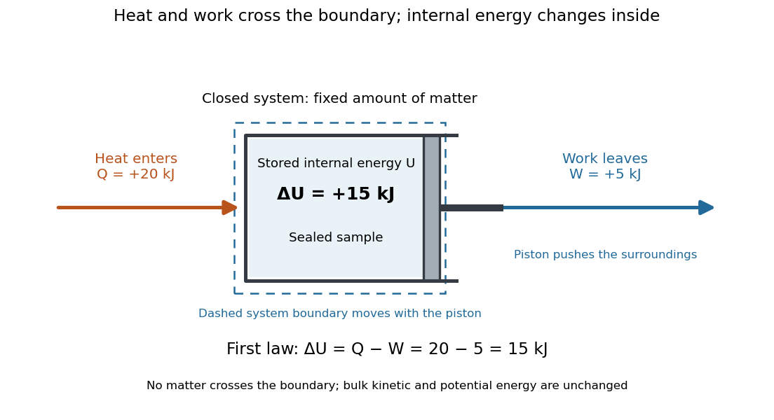

Unlike internal energy, heat is not a state function: different paths between the same equilibrium states can transfer different , with compensating differences in work. The symbol records this dependence on the path; there is no stored quantity whose difference is always . The two paths in first law of thermodynamics illustrate this directly. Supplied heat can raise temperature as sensible heat, change a phase fraction through latent heat, or help supply expansion work. Measuring temperature alone therefore does not determine transferred heat.
For a reversible thermodynamic process, , where is absolute temperature and is entropy. This identification requires reversibility: an irreversible adiabatic process has and can nevertheless increase entropy. Likewise , with enthalpy , requires the particular fixed-pressure conditions in enthalpy. These distinctions make heat useful as a precise boundary-transfer quantity in heat engines, refrigerators and heating calculations.
Historically, James Prescott Joule's paddle experiments showed that stirring water with input work could raise its temperature, helping establish conservation of energy. The lesson is still useful: a temperature rise can result from work even without incoming heat. [ref]
https://openstax.org/books/university-physics-volume-2/pages/1-4-heat-transfer-specific-heat-and-calorimetry. Ling, Moebs and Sanny, OpenStax, section 1.4: Joule's paddle experiment
Heat capacity Created 2026-09-24 Updated 2026-10-14
Heat capacity measures the heat supplied per small temperature increase along a specified process:The subscript records the constraint, such as fixed volume or fixed pressure. The units are . The symbol emphasizes that heat is a transfer along a path, rather than a state function with a differential . Consequently, an unspecified heat capacity does not determine the required heat.
For a closed system of fixed composition undergoing a quasistatic process, assume that only pressure-volume work occurs, with no friction and no change in bulk kinetic energy or potential energy. The first law of thermodynamics and , where is internal energy and is enthalpy, then giveThese partial derivatives define heat capacity at constant volume and heat capacity at constant pressure, with the amount and composition also held fixed. Integrating along the selected constraint gives within a single thermodynamic phase; requires constant . [ref]
For a computed example, take a monatomic gas in the classical ideal gas regime, with amount of substance and stipulated molar gas constant . The equipartition theorem gives , and the ideal gas law gives . ThusFor the same temperature increase , the two processes requireHere work done by the gas is positive. At fixed pressure, the extra heat supplies expansion work; the internal energy increase is the same because internal energy of an ideal gas depends only on temperature. Their final volume values differ. [ref]
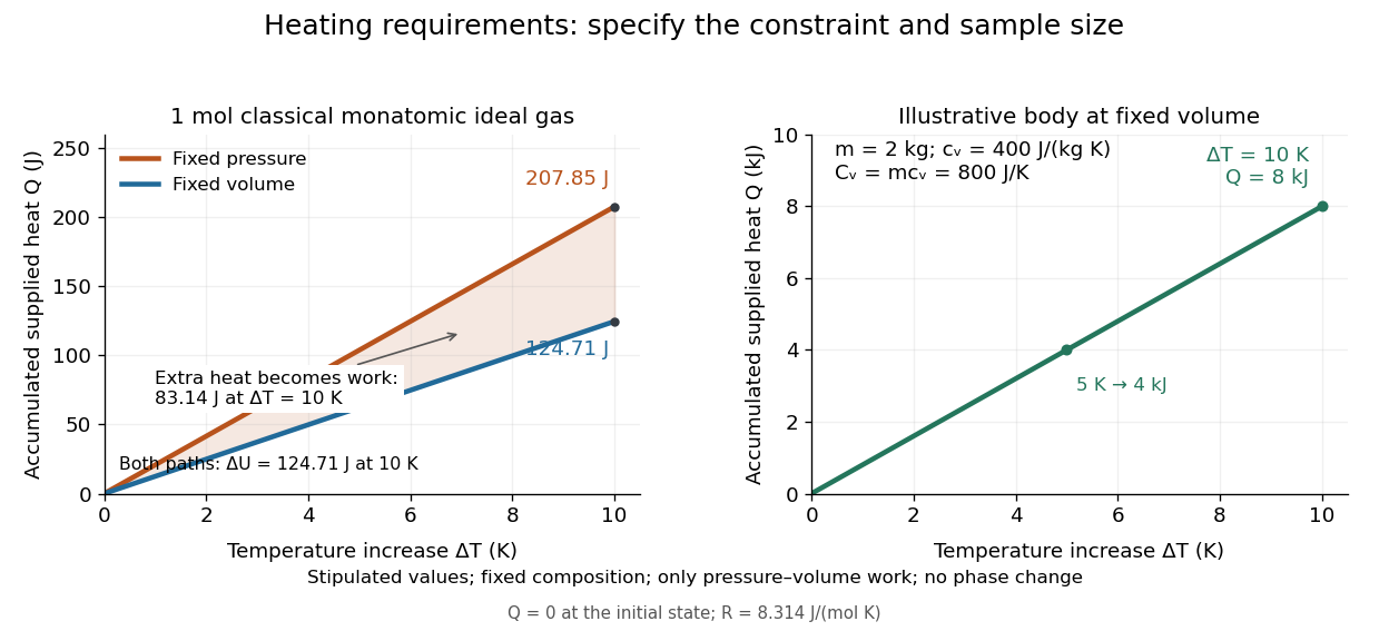
Required heat depends on the constraint and the amount of material
. Left: one mole of classical monatomic gas with the stipulated molar gas constant above; the shaded difference is expansion work at fixed pressure. Right: the illustrative fixed-volume body from specific heat capacity, with mass and . Each curve starts at zero accumulated heat, rather than zero absolute internal energy. Details.
The practical value of heat capacity is that a measured heat input and temperature response can determine it. Once its constraint and temperature dependence are known, it predicts heating requirements and supplies entropy changes through entropy from heat capacity. [ref]
1 The Fundamentals of Statistical Mechanics. Tong, Statistical Physics, heat capacity as a measurable response
Heat capacity at constant pressure Created 2026-09-24 Updated 2026-10-14
For a fixed-composition closed system, the heat capacity at fixed pressure is , with enthalpy . Under the quasistatic process assumptions in heat capacity, only pressure-volume work is permitted, so gives . Thus supplied heat is , or within a single thermodynamic phase when is constant. For an ideal gas, the expansion work explains why this exceeds the required heat at fixed volume for the same temperature increase. Its per-unit-mass counterpart is specific heat capacity at constant pressure.
Heat capacity at constant volume Created 2026-09-24 Updated 2026-10-14
For a fixed-composition closed system, the heat capacity at fixed volume is , with internal energy . Under the quasistatic process assumptions in heat capacity, only pressure-volume work is permitted, so gives . A rigid vessel therefore needs , or when is constant. Its per-unit-mass counterpart is specific heat capacity at constant volume.
Heat engine 2026-10-14
A heat engine uses a repeating thermodynamic cycle to turn part of an incoming heat transfer into net outgoing work. In the two-thermal reservoir model, the hot thermal reservoir supplies heat at fixed temperature , and the cold thermal reservoir receives heat of magnitude at fixed temperature . A Stirling engine makes the repeated motion visible; the abstract energy budget applies independently of its particular mechanism.[ref]
3.2 Generalized Representation of Thermodynamic Cycles. §3.2, Figure 3.3: two reservoirs and net work output
Choose the entire cyclic device as a closed system, with no net change in bulk kinetic energy or potential energy. Count heat entering as positive and net work delivered as positive, as in the first law of thermodynamics. Thus enters with a plus sign and , although a positive magnitude, enters with a minus sign. Assume these two heat transfers and the net work are the only transfers across the boundary. Over one complete thermodynamic cycle, all stored energy, including internal energy , returns to its starting value:The device does not accumulate heat from cycle to cycle. More precisely, heat is a transfer, while internal energy is what can be stored; even a component that temporarily stores internal energy must return to its initial state for this boundary to be cyclic.[ref]
For engine operation, and . Its thermal efficiency isUse net work, after subtracting any work supplied during compression or required by auxiliaries included in the chosen device. For periodic operation, average power satisfies and , with the rates averaged over complete thermodynamic cycles.[ref]
For a stipulated model at and , let and per thermodynamic cycle. Then and . At two thermodynamic cycles per second, these become incoming heat transfer, outgoing heat transfer, and net power. These are constructed values, not measurements.
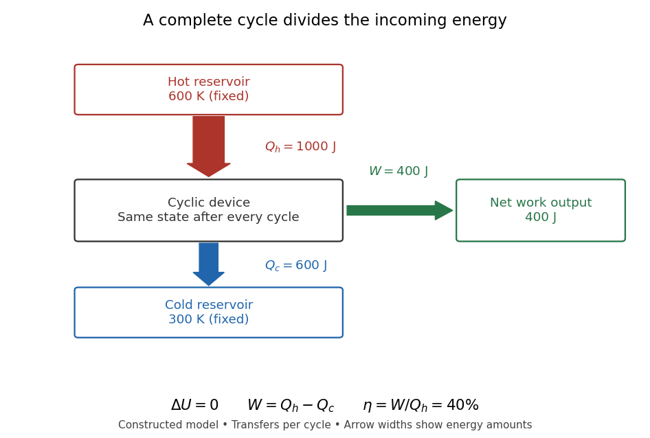

Different signs describe different tasks. With the same directions of heat transfer, gives : a device transmitting heat without net work output. If , net work is supplied to that device. A refrigerator or heat pump instead extracts heat from the cold side and delivers heat to the hot side, using positive input work and the balance . Their useful output is heat transfer, measured by a coefficient of performance. Finally, a one-time isothermal expansion can have and while leaving the volume changed: it is not a complete thermodynamic cycle. A warming device also fails the cyclic assumption, and a fuel-consuming device requires an accounting of matter crossing its boundary.
For two fixed thermal reservoirs at positive thermodynamic temperatures, the Second law of thermodynamics strengthens the energy balance toEquality requires the overall operation to be a reversible thermodynamic process, including its heat transfer to the thermal reservoirs. The Carnot cycle explains how the reversible benchmark is constructed, and Carnot's theorem explains its universality and the entropy production penalty. Use kelvin values, never ratios of degree Celsius readings. The example above lies below the bound: its total entropy production is per thermodynamic cycle.
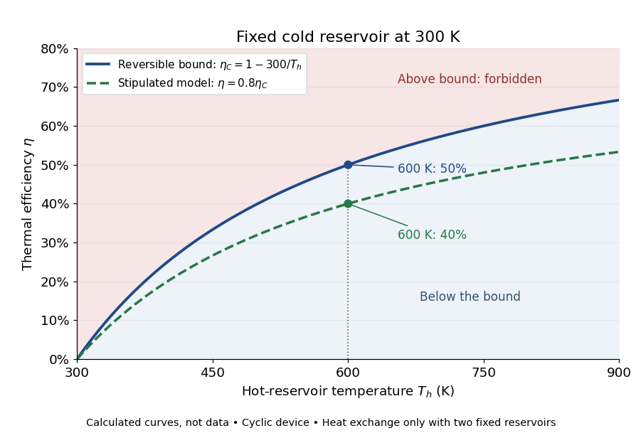

This is useful before building a machine: warmer cooling surroundings reduce the possible thermal efficiency, even if the mechanism is unchanged. A small observed thermal efficiency does not by itself test the Second law of thermodynamics; heat leaks, friction, incomplete recovery of work, and the measurement boundary can all reduce the reported ratio. A meaningful comparison requires the actual thermal reservoir temperatures, matched heat and net work measurements, and the hypotheses of Carnot's theorem. Finite bodies whose temperatures change are treated separately there.
The practical question already appears in the 1824 Réflexions sur la puissance motrice du feu et sur les machines propres à développer cette puissance by Sadi Carnot: pp. 6–8 ask whether machines driven by heat have a fundamental limit and whether changing the working substance can improve their output. Pages 9–11 describe heating and cooling in real machines, but use the historical caloric theory, rather than the modern first law of thermodynamics balance. The historical discussion under Carnot's theorem explains that distinction.
Heat-engine calorimetry 2026-10-14
Heat-engine calorimetry measures heat transfers so that observed work can be compared with the correct energy input. Measuring motion alone cannot supply the denominator of thermal efficiency.
The institutional Laboratory 16: Stirling Engine describes a modern teaching arrangement: an ethanol lamp drives a Stirling engine coupled to an electrical output device, which supplies a resistor immersed in water in a calorimeter. The prescribed readouts include fuel mass consumed, the pressure-volume loop, electrical readings, and water temperature. The sequence separates fuel input, gas-cycle work, electrical output, and Joule heating of the water. Warming of the water is the final useful output; it is not the engine's rejected . The handout distinguishes warm-up from steady operation and asks students to compare the final warming with direct heating by the lamp. It gives a procedure, not a table of measured efficiencies. Its pp. 1–3 therefore establish an apparatus and measurement design without supplying a new experimental result.
For a proposed calibration, use a known input of electrical work to determine the effective heat capacity of the water, vessel and immersed parts; stir to make the measured temperature representative. A matched run with no input estimates exchange with the room. For constant and no phase transition, the resulting model iswhere is the signed net heat lost to the room during the measurement. Here is supplied electrical work when the resistor lies inside the calibration boundary; for a separate external heat input it is the received heat. These are proposed controls, not controls reported in that handout. Slow cooling, changing material properties and imperfectly matched room exchange limit this inference; the approach to thermal equilibrium and heat capacity matter as much as the thermometer reading.
To measure the actual engine-input , one must instrument its hot-side transfer separately, or close a calibrated energy balance around a specified heater boundary. A heater's electrical work includes changes in its stored internal energy and heat transfer that bypasses the engine. At periodic operation a cold-side flowing-water measurement can instead estimate , if mass flow rate and specific heat capacity at constant pressure are known, with negligible storage and other heat exchange in that measurement boundary. It measures only the rejection captured by that stream. Include all remaining transfers before using the residual to infer . This measurement discipline makes a comparison with Carnot's theorem meaningful.
Heat-flow reversal along a thermodynamic path Created 2026-10-20 Updated 2026-11-05
For a quasistatic simple compressible system with only pressure-volume work, the direction of heat transfer is determined by . A reversal occurs where this vanishes and changes sign. It need not coincide with a maximum or minimum of temperature, because the substance can still do work when its internal energy is stationary.
Heat input to a cycle 2026-10-20
The heat input to a cycle sums positive transfers of heat into its working substance. It is not the net heat over the entire cycle, which equals net work. A single geometric branch can contain both heat absorption and rejection, so grouping the branch into one net transfer can overestimate a heat engine's thermal efficiency.
Heat pump 2026-10-14
A heat pump uses work to deliver heat to the region we want to keep warm. Its useful output is the hot-side delivery . The same operating machine can be described as a refrigerator when the cold-side extraction is the objective: which output is useful changes the coefficient of performance, while the energy balance stays . Heating a water bath by taking heat from a colder water bath makes this distinction visible in the heat-pump calorimetry experiment below. [ref]
https://labs.phys.utk.edu/mbreinig/phys136core/modules/m3/refrigerators.html. University of Tennessee, Refrigerators, air conditioners, and heat pumps: heating objective
In the illustrative budget from refrigerator, supplying of work delivers of useful heat, giving a heating coefficient of performance of . The additional came from the colder region. Compare an ideal electrical heater whose entire input work becomes heat in the target region: it delivers for that input. The appeal of a heat pump is this ability to move existing energy, while the Second law of thermodynamics limits the work saving for a given pair of temperatures.
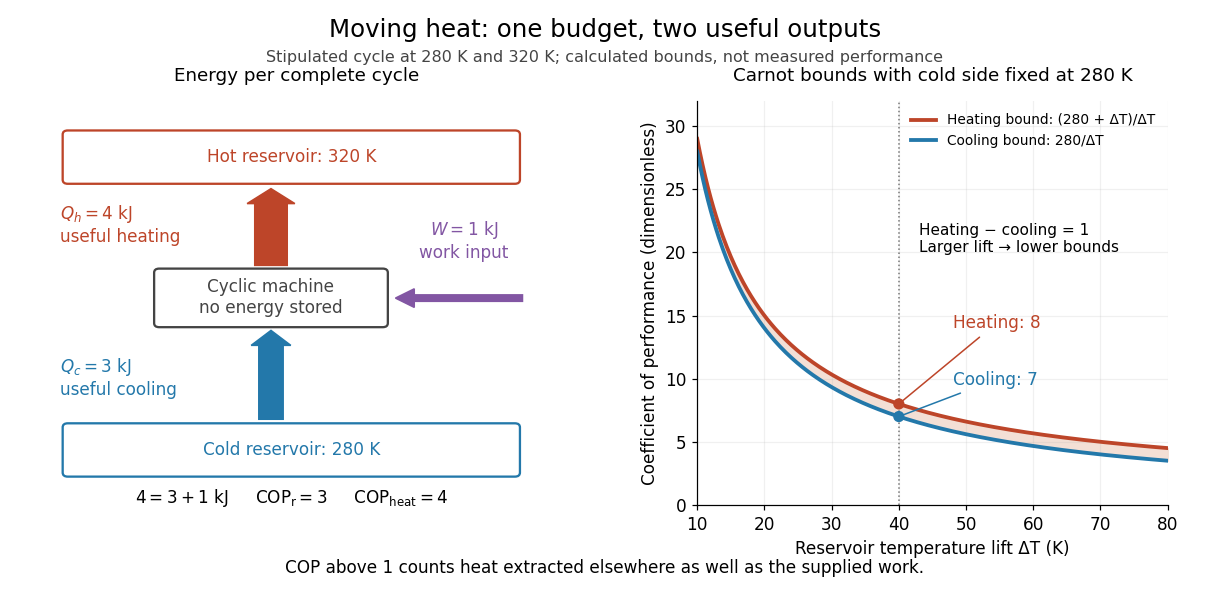
One energy budget, two useful outputs, and Carnot's theorem bounds on the coefficient of performance
. Original quantitative diagram, with stipulated , and . Arrow widths follow the transfer magnitudes. The curves are reversible bounds for fixed cold temperature and varying hot temperature ; they are not measured performance. At , the bounds are for cooling and for heating, above the illustrative machine's and . Details.