The conjugate exponent of $1<p<\infty$ is $q=p/(p-1)$, so $1/p+1/q=1$. The endpoint conventions pair $1$ with $\infty$ and $\infty$ with $1$. Examples are $(p,q)=(2,2)$, $(3,3/2)$ and $(4,4/3)$. The exponents themselves need not add to one; their reciprocals do.

A Hohmann transfer orbit between coplanar circular Kepler orbits of radii $r_1,r_2$ traverses half an elliptic orbit of semi-major axis $a=(r_1+r_2)/2$. Kepler's third law therefore gives $t=\pi \sqrt{a^3/(GM)}$. Relative to the initial orbital period $T_1$, $t=(T_1/2)[(r_1+r_2)/(2r_1){]}^{3/2}$. Radii must be measured from the attracting centre, rather than from its surface.

For a Hohmann transfer orbit from radius $r_0$ to $\eta r_0$, with $\eta >1$ and initial circular speed $v_0=\sqrt{GM/r_0}$, conservation of orbital energy and angular momentum gives transfer endpoint speeds $v_p/v_0=\sqrt{2\eta /(1+\eta )}$ and $v_a/v_0=\sqrt{2/[\eta (1+\eta )]}$. The required prograde impulses areIf the spacecraft mass is constant and fuel use is proportional to impulse magnitude, these also give the fuel fractions relative to a budget with total speed change $v_0$. Their sum is a sum of magnitudes, even though the burns occur at different positions and directions.

For an original classical calculation of the return step, neglect the residual ion's Coulomb force after release. Take a spatially uniform driving electric field $E(t)=E_0\cos \omega t$, an electron of electric charge $-e$ and mass $m$, and zero initial position and velocity at $t_i$. With $\alpha =\omega t_i$ and $\beta =\omega t$, integrating Newton's second law givesA return requires $\beta >\alpha$ and $x(t)=0$. Define the cycle-averaged free-electron quiver kinetic energySearching the first-return solutions for release phases $0<\alpha <\pi /2$ gives a maximum near $\alpha =0.3134$ and $\beta =4.3990$, with $K_{\mathrm{return}}\simeq 3.1731U_p$. For a chosen ionization energy $I_p$, recombination into the initial state can therefore emit a photon with energy up to approximately $I_p+3.17U_p$ in this model. This is an upper return-energy scale, not a prediction of the emitted yield. It omits release probabilities, quantum interference, propagation, phase matching and depletion of the neutral gas.

The calculation explains why a long driving wavelength can increase the available return energy: at fixed $E_0$, $U_p$ grows as ${\omega }^{-2}$. It does not say that conversion efficiency improves. The electron must return with a probability amplitude for emission that survives the microscopic dynamics and adds coherently across the gas.

For the physicists' Hermite polynomials $H_n=(-1{)}^n{e}^{x^2}{D}^n{e}^{-x^2}$, the displayed recurrence holds for $n\ge 1$, while $H_0^{\prime }=0$ separately. Put $u=e^{-x^2}$. Differentiating $u^{\prime }+2xu=0$ exactly $n$ times using the Leibniz rule yieldsDifferentiating the defining product for $H_n$ then givesThe nonnegative integer convention is essential for the derivative-based definition; no negative-order derivative or $H_{-1}$ is needed.

The potential energy $V(x,y)=\frac{1}{2}(x^2+y^2)+x^{2}y-y^3/3$ in the Hénon-Heiles system has the following expression in polar coordinates:so it is invariant under rotation through $2\pi /3$. Solving $\nabla V=0$ gives a strict local minimum at the origin and three saddle points, at $(0,1)$ and $(\pm \sqrt{3}/2,-1/2)$. All three saddle points have value $1/6$. Their common level set factors exactly:Thus this level set is the union of the three lines $y=-1/2$ and $y=1\pm \sqrt{3}x$. They bound an equilateral triangle containing the local minimum. The Hessian matrix is the identity at the origin; at each of the other three stationary points it has eigenvalues $3$ and $-1$. For energies $0\le E<1/6$, the central accessible region is bounded; above that value the three saddle passages allow paths from the centre to arbitrarily large radius. This follows directly from the radial potential: in each direction with $\sin (3\theta )<0$, its radial maximum occurs at $r=-1/\sin (3\theta )$, with value $1/[6{\sin }^2(3\theta )]\ge 1/6$.

For a closed hemisphere of radius $a>0$, take a rectangular parallelepiped with a face on the flat base, base half-widths $x,y>0$ and height $z>0$. Its curved-boundary constraint is $x^2+y^2+z^2=a^2$ and its volume is $4xyz$. A Lagrange multiplier gives $x=y=z=a/\sqrt{3}$, yielding the displayed maximum. The full edge lengths are $2a/\sqrt{3},2a/\sqrt{3},a/\sqrt{3}$.

This bound remains valid when arbitrary orientations are allowed. Write a cuboid's half-edge lengths as $u_1,u_2,u_3$, its center components in its orthonormal edge basis as $v_i$, and the vertical unit-vector components as $n_i$. Containment above the base plane requires $\sum n_i{v}_i\ge \sum |n_i|u_i$. Hence $|v_j|\ge u_j$ for at least one $j$: otherwise every contributing term would be strictly smaller than its required bound. Its farthest vertex has squared distanceContainment in the sphere bounds the right side by $a^2$. The arithmetic-geometric mean inequality then gives $2u_1{u}_2{u}_3\le a^3/(3\sqrt{3})$, so the full volume $8u_1{u}_2{u}_3$ cannot exceed the displayed value. The constructed cuboid attains it. With strict containment and no boundary contact, the same value is a supremum.

Use the coordinate conventionIn this convention the Heisenberg group over a prime field has the productThe subset $H=\{A(t,b,t):t,b\in {\mathbb{F}}_p\}$ is an Abelian subgroup of order $p^2$: the middle coordinate in a product is $b+b^{\prime }+t{t}^{\prime }$, which is symmetric in the factors. Also $A(t,b,t{)}^{-1}=A(-t,t^2-b,-t)$ lies in $H$. The map $A(a,b,c)\mapsto a-c$ is a surjective group homomorphism to the additive group of ${\mathbb{F}}_p$, with kernel of a group homomorphism $H$. Hence $H$ is a normal subgroup of subgroup index $p$, and its left cosets are exactly the level sets of $a-c$.

For odd $p$, an explicit group isomorphism from $H$ to the additive group ${\mathbb{F}}_p^2$ isThe term $t{t}^{\prime }$ in matrix multiplication cancels the cross term in $(t+t^{\prime }{)}^2/2$. Thus $H$ is an elementary abelian group, isomorphic to $C_p\times C_p$.

A heat sink receives thermal energy from a component and provides a path for exporting it to a surrounding fluid or another reservoir. A metal block can spread a localized heat load by thermal conduction; fins enlarge the surface available for convection and thermal radiation. The entire path also includes the thermal resistance of the contact between component and heat sink.

For a simplified steady linear model, a component dissipating power $P$ sits above the ambient temperature by $\Delta T=P{R}_{\mathrm{th}}$, with total thermal resistance $R_{\mathrm{th}}$. Increasing a block's heat capacity can slow its transient warming but does not by itself lower this final temperature rise. This distinction can be tested with a fixed-power heating step: the early slope probes storage, while the long-time rise probes transport. A heat sink therefore needs an effective route to the environment as well as material that conducts heat internally.

A heat current is the rate of heat transfer across a specified oriented boundary, $\dot{Q}$, measured in watts. For a heat flux field $\mathbf{q}$ and outward unit normal vector $\mathbf{n}$, the outward heat current through a surface isThe sign convention matters: outward and inward currents for the same physical transfer have opposite signs.

A uniform normal heat flux $100\mathrm{W}{\mathrm{m}}^{-2}$ through $0.02{\mathrm{m}}^2$ gives a heat current of $2\mathrm{W}$. Maintaining it for $30\mathrm{s}$ transfers $60\mathrm{J}$. In steady one-dimensional thermal conduction without internal sources, the current is constant along a bar even if changing cross-sectional area makes the local heat flux vary. This separates a whole-path transport rate from its concentration over a surface.

On $0<x<a$, $0<y<b$, impose zero Dirichlet boundary conditions at $x=0,a$ and zero Neumann boundary conditions at $y=0,b$. Separation of variables for $T_t=\lambda \Delta T$ gives the displayed sine-cosine expansion. The zero cosine mode must be included: its norm is $b$, whereas the positive cosine modes have norm $b/2$. Thus $A_{n0}=2(ab{)}^{-1}\int \int T_0\sin (n\pi x/a)$ and $A_{nm}=4(ab{)}^{-1}\int \int T_0\sin (n\pi x/a)\cos (m\pi y/b)$ for $m\ge 1$. Expanding $x(a-x)$ gives sine coefficient $4a^2[1-(-1{)}^n]/(n^3{\pi }^3)$. Initial data $x(a-x){\sin }^2(2\pi y/b)$ therefore involve only $m=0,4$ and odd $n$. Their leading long-time mode is $4a^2\sin (\pi x/a)e^{-\lambda {\pi }^{2}t/a^2}/{\pi }^3$.

For a diffusion equation with fixed homogeneous boundary conditions, a fundamental diffusion mode is an eigenfunction of its nonnegative decay operator belonging to the smallest decay eigenvalue ${\nu }_0$, when such an eigenvalue exists. It is the slowest decaying separated normal mode. With a discrete spectrum and an isolated lowest eigenvalue, initial data having a nonzero projection onto its eigenspace approach this decay law at late times. Strongly vanishing thermal diffusivity can destroy existence of a lowest mode, as illustrated by the loss of a spectral gap under strongly degenerate radial diffusion.

For a long homogeneous circular wire of radius $a$, uniform volumetric heating $H$, constant thermal conductivity $\kappa$ and negligible end losses, the steady heat equation is $\kappa {\rho }^{-1}(\rho T^{\prime }{)}^{\prime }+H=0$. Regularity at the axis excludes a logarithm term, giving $T=T_s+H(a^2-{\rho }^2)/(4\kappa )$. If the surface obeys Newton's law of cooling, $-\kappa T^{\prime }(a)=\gamma (T_s-T_{\mathrm{air}})$, then $T_s=T_{\mathrm{air}}+Ha/(2\gamma )$. Here $\gamma$ has units $\mathrm{W}{\mathrm{m}}^{-2}{\mathrm{K}}^{-1}$ and $H$ has units $\mathrm{W}{\mathrm{m}}^{-3}$. For uniform electric current $I$ and constant electrical conductivity $\sigma$, Joule heating gives $H=I^2/(\sigma {\pi }^2{a}^4)$.

On $0<x<L$, let $u_t=\nu u_{xx}+G\sin (n\pi x/L)$, with $\nu >0$, zero Dirichlet boundary conditions, and zero initial data. Write $k_n=n\pi /L$. Its stationary solution is $u_s=G\sin (k_{n}x)/(\nu k_n^2)$. Subtracting it removes the forcing from the partial differential equation and leaves a heat equation with initial data $-u_s$.

Because the forcing is a single spatial eigenfunction, separation of variables gives the entire solution without mixing modes:Its integral is $G[1-(-1{)}^n](1-e^{-\nu k_n^{2}t})/(\nu k_n^3)$; even modes have zero signed net integral. Removing forcing from the evolution equation does not remove its amplitude from the initial data for the transient.

For a circle of circumference $2\pi$, the heat equation $u_t=D{u}_{xx}$ has periodic matching of both $u$ and $u_x$ at $x=\pm \pi$. For $D>0$, the displayed Fourier series solves the initial-value problem, with $\bar{f}=(2\pi {)}^{-1}{\int }_{-\pi }^{\pi }f(x)dx$ and the usual real Fourier coefficients. Every nonconstant normal mode decays, leaving the conserved mean. In particular $f(x)=(\pi -|x|{)}^2$ gives $\bar{f}={\pi }^2/3$, $a_n=4/n^2$ and $b_n=0$. The initial cusp is smoothed for every positive time.

The contribution of electrons to heat capacity. For a uniform noninteracting three-dimensional Fermi gas at fixed particle number and volume, its low-temperature value is $C_V\simeq ({\pi }^2/2)N{k}_{B}T/T_F$; only states near the Fermi surface can change occupation readily.

A Schottky anomaly is a peak in heat capacity caused by thermal occupation of a small set of separated energy levels. For $N$ independent two-level units with equal degeneracies and gap $\Delta >0$, write $x=\Delta /(k_{B}T)$; their heat capacity is $C=N{k}_B{x}^2{e}^{-x}/(1+e^{-x}{)}^2$, with Boltzmann constant $k_B$. It vanishes at both low and high temperature and can spoil a lattice $T^3$ fit in between. Localized electronic or nuclear levels can contribute, including in calorimeter addenda; their presence must be checked rather than attributed automatically to phonons.

Electronic heat capacity is the contribution from electronic excitations to heat capacity. A simple normal metal with a smooth density of states near its Fermi energy has $C_{\mathrm{m}}^{\mathrm{el}}\simeq \gamma T$ well below its electron Fermi temperature. Only a narrow energy interval near the Fermi energy changes occupation on heating, explaining the small fraction of active electrons. The Debye T-cubed test separates this contribution from lattice phonons. Interactions, a superconductivity transition or other electronic structure can invalidate a constant $\gamma$ description.

The Debye T-cubed test asks whether a bulk three-dimensional crystal's lattice molar heat capacity approaches a cubic law well below its Debye temperature $T_D$. It tests the low-frequency acoustic phonon branches in the Debye model, rather than asserting that every contribution to a real sample's heat capacity is cubic. Peter Debye's continuum description makes a striking connection: a thermal measurement can reveal the low-frequency vibrational density of states without resolving individual vibrations.^[ref]

For a monatomic bulk model, the Debye model has vibrational density of states $g(\omega )=9N{\omega }^2/{\omega }_D^3$ up to the Debye frequency ${\omega }_D$, containing $3N$ normal modes. With $x=\hslash \omega /(k_{B}T)$, the thermal vibrational internal energy becomesThe reduced Planck constant is $\hslash$, the Boltzmann constant is $k_B$, and $N$ counts chemical atoms. For $T\ll T_D$, replace the upper limit by infinity. The integral is ${\pi }^4/15$, as in the Stefan–Boltzmann law derivation. Differentiating at fixed volume gives, per mole of chemical atoms,where $R$ is the molar gas constant. The cubic exponent comes from three-dimensional acoustic phonon branches with linear low-wavevector dispersion relations. The coefficient encodes their propagation speeds. Formula-unit normalization in a compound requires its number of chemical atoms per formula unit; do not silently substitute moles of formula units for moles of chemical atoms.

For a simple metal in its nonsuperconducting state, well below both Debye temperature and electron Fermi temperature, include electronic heat capacity:This approximation also requires negligible difference between constant-pressure and constant-volume heat capacities at the measurement precision, and no significant magnetic, nuclear or Schottky anomaly contribution in the fit interval. Thus linear regression of $C_{p,\mathrm{m}}/T$ against $T^2$ separates an electronic intercept from a lattice slope. For an insulating crystal with no relevant low-energy magnetic excitations, the electronic term can instead be negligible; a superconductivity transition changes the electronic response.^[ref]

After subtracting calorimeter addenda, Brando's second gold sample, $72.6\mathrm{mg}$, gave a linear $C_{p,\mathrm{m}}/T$ versus $T^2$ plot in the nonsuperconducting state. The reported electronic intercept was $7.0\times 10^{-4}\mathrm{J}\mathrm{mo}{\mathrm{l}}^{-1}{\mathrm{K}}^{-2}$; deviations from reference heat capacities were below $2\%$.^[ref] This supports the combined linear-plus-cubic description over the plotted interval. Because the platform subtraction used reference gold, it is also an instrument validation with a shared material standard, rather than a wholly independent determination of the Debye model from an uncalibrated instrument.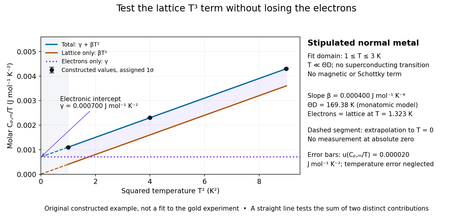

For a worked original inference, stipulate values of $y=C_{p,\mathrm{m}}/T$ equal to $(0.001100,0.002300,0.004300)\mathrm{J}\mathrm{mo}{\mathrm{l}}^{-1}{\mathrm{K}}^{-2}$ at $T=(1,2,3)\mathrm{K}$. Assign independent $u(y)=0.000020\mathrm{J}\mathrm{mo}{\mathrm{l}}^{-1}{\mathrm{K}}^{-2}$ and negligible temperature error. Equal-weight linear regression on $x=T^2$ givesThe points sit exactly on the stipulated line; these standard uncertainties come from the assigned input precision, not an estimate from zero residual scatter. With $R=8.314462618\mathrm{J}\mathrm{mo}{\mathrm{l}}^{-1}{\mathrm{K}}^{-1}$, inversion givesAt $2\mathrm{K}$, the electronic and lattice molar heat capacities are respectively $0.0014$ and $0.0032\mathrm{J}\mathrm{mo}{\mathrm{l}}^{-1}{\mathrm{K}}^{-1}$. Their equality occurs at $\sqrt{\gamma /\beta }=1.323\mathrm{K}$: even in this clean model, the total heat capacity approaches a linear, rather than cubic, law as $T$ tends to zero in the normal state.

A straight line over a narrow interval is a useful diagnostic, not a universal proof. Inspect residuals and repeat the fit over several upper and lower temperature cutoffs; curvature can signal higher lattice terms, an unremoved Schottky anomaly, or a faulty calorimeter addenda subtraction. Correlated thermometer calibration and sample-amount errors affect both axes and can dominate the illustrative linear regression uncertainty. Low-dimensional samples, additional low-energy excitations and proximity to a phase transition need other models. The test is valuable precisely because its failures can reveal physics beyond the bulk acoustic approximation.

Low-temperature calorimetry measures a small sample's heat capacity by resolving a small temperature change after a known electrical energy input. The experimental challenge is that the support, heater and thermometer also warm up. Their calorimeter addenda must be removed before interpreting the sample's phonons or electronic heat capacity. The Debye T-cubed test turns the corrected response into a test of the low-temperature vibrational spectrum.

Manuel Brando's 2009 experiment used a sapphire platform suspended by four alloyed platinum wires from a copper ring fixed to a cryostat stage. Grease attached the sample; a chip heater and ruthenium-oxide resistance thermometer served platform PLS-2. A controller stabilized the bath; a lock-in amplifier supplied heating pulses and read the calibrated sensor. The steady rise calibrated thermal conductance as $G=P/\Delta T$. A separate $59.1\mathrm{mg}$, $99.99\%$ pure gold sample, compared with reference heat capacities, established the calorimeter addenda. Small pulses limited property variation; imperfect sample contact required a second relaxation time. The platform contribution rose below $1.5\mathrm{K}$, making simple extrapolation unsafe.^[ref]

For an original idealization, assume sample and platform share one temperature $T$, the bath remains at $T_b$, and both the total heat capacity and the weak-link thermal conductance $G$ are approximately constant across one small pulse. Ignore other heat transfer and any phase transition. The first law of thermodynamics becomesHere $C_s$ is sample heat capacity, $C_a$ is calorimeter addenda, $P$ is deposited electrical power from Joule heating, and $\tau$ is a time constant. This is the same balance as calorimeter heat-loss correction, used here with a deliberately weak cryogenic link and a separately subtracted platform. For a constant pulse $P_0$ beginning at bath temperature, then switched off at $t_h$,The cooling exponential decay determines $\tau$, while the heating plateau determines $G=P_0/(T_{\infty }-T_b)$. Together with calorimeter addenda, they give $C_s=G\tau -C_a$. Cooling alone determines a ratio, not an absolute heat capacity. With finite $t_h$, the observed end rise is smaller than the plateau; fit the full response or apply the displayed correction rather than identifying the two.

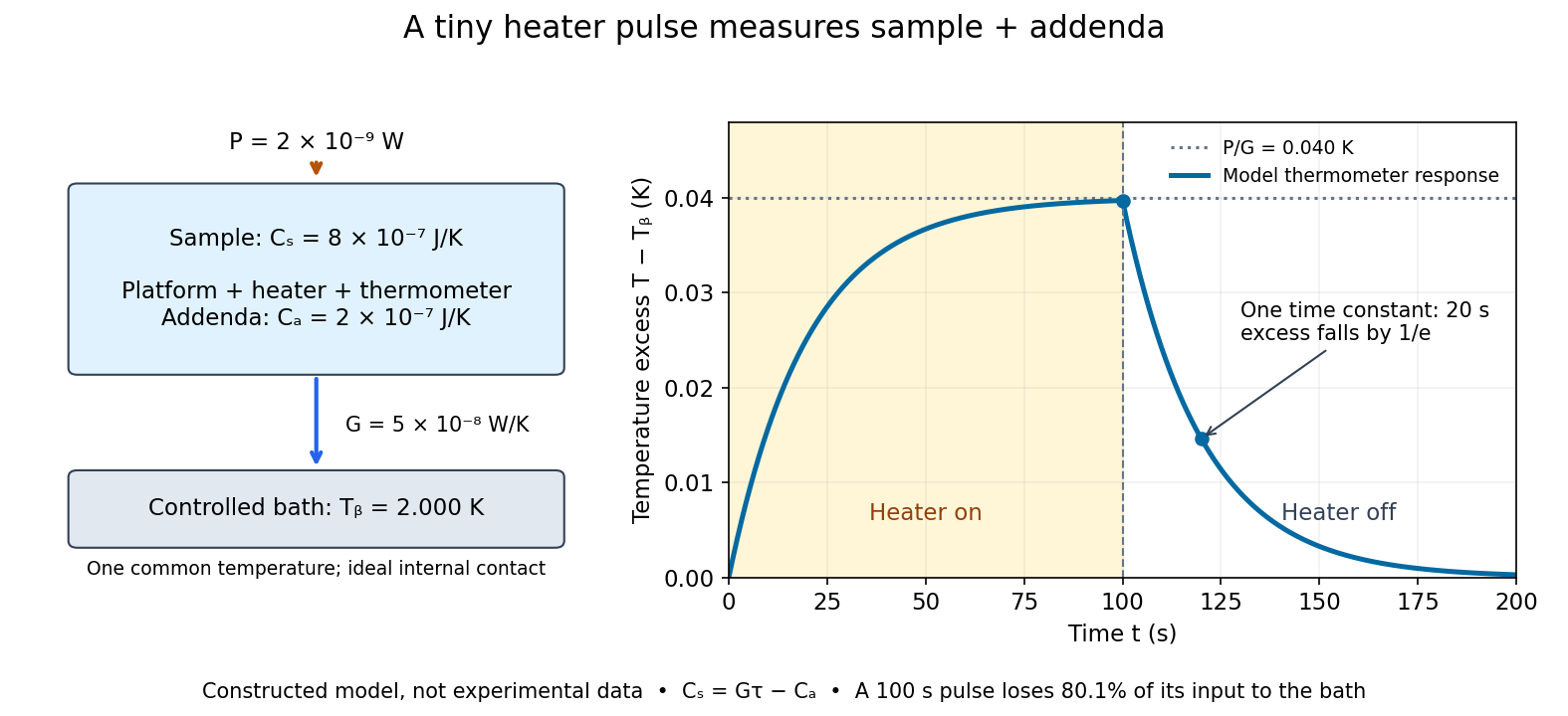
For the stipulated figure parameters, $G=5.00\times 10^{-8}\mathrm{W}{\mathrm{K}}^{-1}$, $\tau =20.0\mathrm{s}$, and $C_a=2.00\times 10^{-7}\mathrm{J}{\mathrm{K}}^{-1}$ give $C_s=8.00\times 10^{-7}\mathrm{J}{\mathrm{K}}^{-1}$. The asymptotic rise is $0.0400\mathrm{K}$, only $2\%$ of bath temperature. At $100\mathrm{s}$, the rise is $0.0397305\mathrm{K}$. Of $2.00\times 10^{-7}\mathrm{J}$ input, only $3.97305\times 10^{-8}\mathrm{J}$ remains stored: the other $1.60270\times 10^{-7}\mathrm{J}$ has flowed to the bath. Treating this long pulse as an isolated $Q/C$ experiment would overestimate total heat capacity by a factor of $5.034$.

Suppose independent standard uncertainties are $u(G)=0.05\times 10^{-8}\mathrm{W}{\mathrm{K}}^{-1}$, $u(\tau )=0.2\mathrm{s}$ and $u(C_a)=0.10\times 10^{-7}\mathrm{J}{\mathrm{K}}^{-1}$. First-order propagation of uncertainty givesThe uncertainty is one standard deviation under those assumptions, about $2.2\%$ of sample heat capacity. Shared thermometer calibration errors can correlate fitted $G$ and $\tau$; then their covariance contributes too. Smaller samples amplify the relative influence of calorimeter addenda. Proposed checks include varying pulse amplitude, repeating with a reference sample, checking sensor self-heating, and comparing single- and two-time-constant fits. A drifting bath, slow internal equilibration or a transition invalidates this simple reduction even if a cooling curve looks smooth.