The cosmic microwave background is nearly isotropic thermal electromagnetic radiation. Its spectrum connects radio receiver measurements with the universe's thermal history: redshift preservation of a thermal photon spectrum cools a blackbody spectrum as space expands. The 1965 Princeton analysis described this relation.[ref]
Cosmic Black-Body Radiation by R. H. Dicke and others. pp.415–416: expansion cools radiation while preserving a thermal spectrum
A radiometer cannot label a received photon as cosmic, atmospheric or instrumental. Its measured power combines the incoming radiation with the receiver response. The useful question is which comparisons and controls can isolate a sky contribution. This makes the Penzias-Wilson microwave background experiment an example of both observational cosmology and measurement calibration.
In 1965, Arno Penzias and Robert Woodrow Wilson reported measurements with a 20-foot horn-reflector antenna at . They manually switched a traveling-wave maser receiver between the horn and a helium-cooled reference. From zenith antenna temperature, atmospheric and antenna/ground contributions left an excess .[ref]
A Measurement of Excess Antenna Temperature at 4080 Mc per Second by Arno Allan Penzias and Robert Woodrow Wilson. pp.419–420: apparatus, temperature contributions and residual
Elevation scans estimated the atmospheric term. Taping horn seams produced no measurable change; a nearby transmitter tested ground response. These controls addressed distinct possible contaminations.[ref]
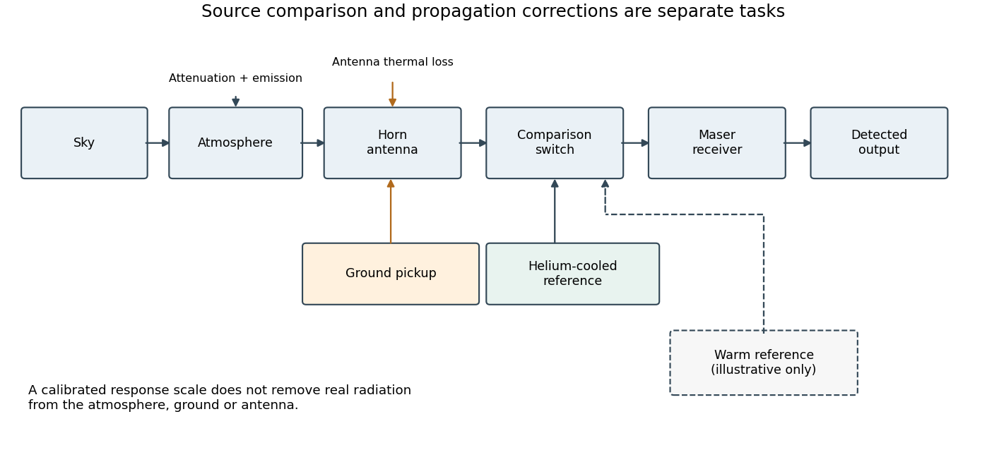
The comparison does not make all nuisance contributions disappear. A reference can establish a response scale, but atmospheric emission and pickup through unwanted antenna directions are also real incident radiation. In his later account, Robert Woodrow Wilson describes these competing contributions as central to a radio astronomy measurement.[ref]
The Cosmic Microwave Background Radiation by Robert Woodrow Wilson. 1978 lecture, introduction and sectionII: sky, ground, atmosphere and instrument contributions
The Princeton group proposed primordial thermal radiation as an interpretation and called for more wavelength measurements. Their separate radiometer had not yet produced results.[ref]
Cosmic Black-Body Radiation by R. H. Dicke and others. pp.415–416: interpretation, Princeton apparatus and need for further wavelengths
A single-frequency excess therefore does not by itself establish a complete Planck spectrum. Reproducibility across independent instruments, observing directions and frequencies tests the interpretation further.Consider an original idealized narrow-band model for one matched spatial mode and one polarization of waves. In the classical Rayleigh-Jeans law regime, an available thermal power can be written , where is the effective bandwidth and the equivalent input noise temperature. Assume a linear detector with stable positive gain and absorb its bandwidth, Boltzmann constant and response factor into . Then the output is , with input-referred receiver noise temperature . These are model assumptions, not a reconstruction of the historical electronics.
Two references with known noise temperatures giveso the two-load radiometer calibration yieldsSubtracting the reference equations eliminates the unknown receiver term; substituting back determines it. An arbitrary stable output offset can likewise be eliminated from the interpolation for , although separating that offset from then requires additional information.
For deliberately chosen inputs, set , , and . These are equivalent noise temperatures; physical load thermometry must be converted consistently at the observing frequency. The reference outputs are and . A sky-input output gives . If independent estimates assign to atmosphere, to antenna loss and to ground pickup in this lumped additive model, the residual is .
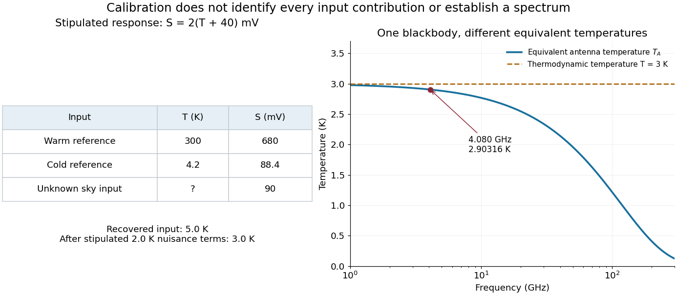
Original calibration arithmetic and the distinction between an antenna temperature and a thermodynamic temperature
. Chosen reference temperatures, receiver response and additive contributions; none are fitted historical measurements. The final panel calculates the Rayleigh-Jeans law equivalent antenna temperature of a stipulated blackbody. A change in frequency changes that equivalent temperature even though the underlying thermodynamic temperature is fixed. Details.The subtraction exposes what a noise budget must achieve. A error in the assigned atmospheric term becomes a error in the residual, even with exact detector calibration. Multiplicative attenuation requires a different correction: if an isothermal atmosphere has transmission , its ideal contribution is in the same classical equivalent-temperature convention. Recovering then requires both subtracting atmospheric emission and dividing by . The additive toy budget applies when its terms already refer to the same receiver input.
There is also a conditioning issue. If is small, a fixed output error strongly changes the inferred temperature. Widely separated reference temperatures improve the scale determination only if the receiver remains linear over that range; measuring the reference repeatedly tests stability rather than proving linearity. The experiment therefore motivates a model, a calibration and a set of independent checks, each with its own assumptions.
For a matched receiver accepting one spatial mode and one polarization of waves, the thermal contribution to the available spectral power of a blackbody isThis expression excludes a zero-point term; it is the thermally emitted contribution. Defining the Rayleigh-Jeans law equivalent antenna temperature by gives the displayed relation. With ,Thus requires . It is an approximation with a frequency-dependent error, rather than a redefinition of thermodynamic temperature.
For the stipulated and , and . Replacing by here would differ by about . At much higher frequencies, the approximation fails more strongly. A real instrument averages over its measured frequency response and antenna beam pattern, so using a single central frequency adds a narrow-band approximation.
The Cosmic Background Explorer connected two questions: does the cosmic microwave background follow a Planck spectrum, and how does its temperature vary across the sky? John C. Mather and George F. Smoot shared the 2006 Nobel Prize in Physics for these discoveries.[ref]
George F. Smoot – Facts by Nobel Prize Outreach. 2006 award and discovery summary
The FIRAS and COBE DMR comparisons below explain why measuring spectral shape and measuring angular structure require different information.FIRAS compared sky radiation with an adjustable internal blackbody using an interferometer and cold bolometers. An external blackbody could cover the sky entrance for measurement calibration. The team adjusted the internal temperature to minimize the difference signal.[ref]
Nobel Lecture: From the Big Bang to the Nobel Prize and beyond by John C. Mather. §III.D, pp.1337–1338; §V.A, p.1341
Comparisons across detectors and mirror strokes tested instrumental errors; sky mapping separated Milky Way emission. John C. Mather's lecture reports a final root-mean-square spectral departure of 50 parts per million of peak brightness. This is neither the preliminary 1990 precision nor a relative error in every spectral bin. Calibration drift and nonideal reference emission required correction.[ref]
Nobel Lecture: From the Big Bang to the Nobel Prize and beyond by John C. Mather. §V.A, p.1342: calibration checks and final spectrum
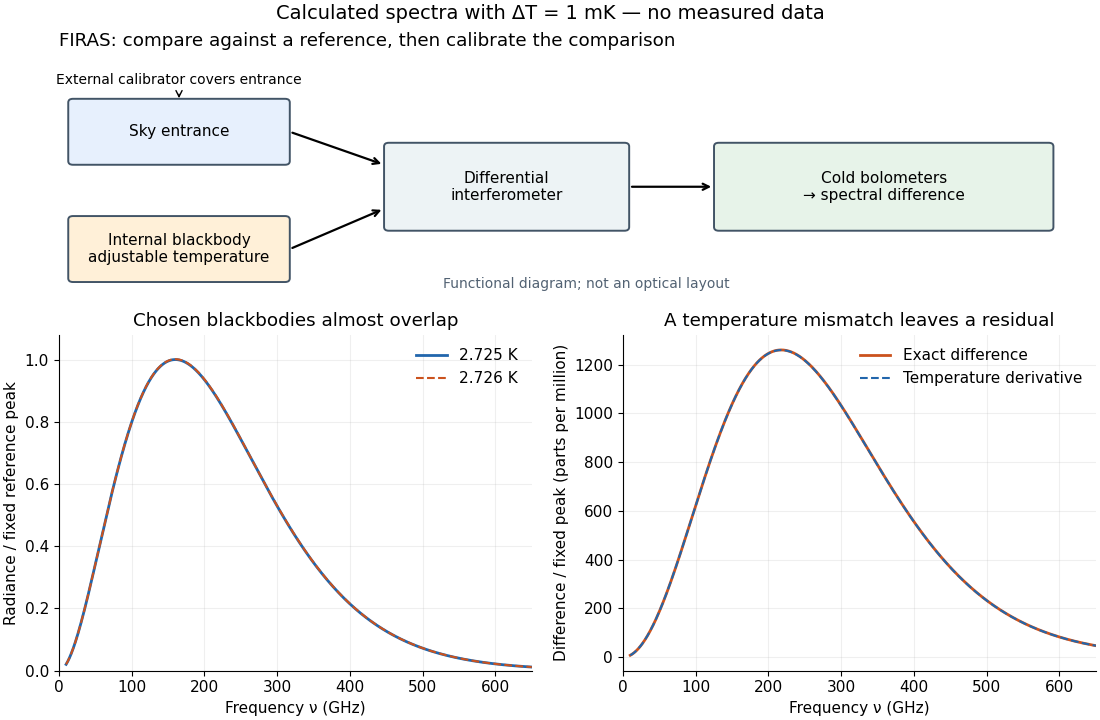
The advantage of a null measurement is that a small difference can be resolved without assigning the same absolute precision to a large detector output. Nevertheless, matching an internal reference is meaningful only after its relation to an independently calibrated blackbody has been tested. A bound on departures from a Planck spectrum constrains energy redistribution after thermal equilibrium; it does not require the cosmic microwave background to have exactly the same temperature in every direction.
For a Planck function expressed as spectral radiance per frequency interval, is the Planck constant, the speed of light and the Boltzmann constant. Differentiating at fixed frequency givesThe proof uses and the chain rule. At low frequency, the multiplier tends to one, recovering the Rayleigh-Jeans law. At high frequency it grows approximately as : the same fractional temperature change has a larger fractional brightness effect on the declining spectral tail.
For an original example choose and . At , , so the first-order fractional residual is . At , , it is . Both spectra are exact blackbodies: this residual is a temperature mismatch, not evidence of a nonthermal spectrum. Fitting temperature before assessing remaining spectral residuals therefore removes a physically distinct degree of freedom. The figure divides by a fixed peak brightness rather than by the rapidly vanishing high-frequency tail.
Hot Electrons in galaxy clusters scatter photons of the cosmic microwave background, producing a characteristic spectral distortion. The thermal contribution measures a line-of-sight integral of Electron pressure, whereas X-ray emission depends approximately on the integral of Electron density squared times a temperature-dependent emissivity. Combining the two with a geometrical model can constrain a cluster's physical size and hence its angular diameter distance. Temperature structure and departures from the assumed geometry introduce systematic uncertainty.
For a uniform spherical cluster of depth , thermal bremsstrahlung gives received bolometric flux , while the Rayleigh-Jeans law limit of the thermal Sunyaev-Zeldovich effect gives . Eliminating and using yields the displayed angular diameter distance. A model for the density profile fixes its numerical coefficient. Clumping, nonsphericity and temperature structure can bias this distance because the two observables weight the gas differently.
Bulk motion of a scattering electron cloud relative to the cosmic microwave background gives a first-order Doppler temperature shift. With positive directed away from the observer, the displayed sign applies, and is the Thomson scattering optical depth. In the nonrelativistic, single-scattering limit it has the spectrum of a small blackbody temperature change, unlike the thermal Sunyaev-Zeldovich effect.
For a Planck photon distribution, the hot-electron Kompaneets equation gives , where . The equivalent thermodynamic temperature perturbation has the displayed form, while the Rayleigh-Jeans law gives . The distortion changes sign at . This first-order expression assumes a small Compton y parameter and nonrelativistic thermal Electrons.
The cosmic microwave background temperature is about , corresponding to the displayed thermal energy. The conversion uses . Thus would correspond to about , rather than the present CMB. Primary references are NASA's CMB temperature measurements and NIST's Boltzmann constant in electronvolts per kelvin.
Reionization returns some neutral cosmic gas to an ionized state after cosmological recombination. The resulting free electrons increase the cosmological optical depth through Thomson scattering and create a second contribution to the cosmological visibility function.
For full hydrogen ionization after instantaneous reionization, and . Integrating Thomson scattering givesFor , . At fixed baryon density and redshift, lowering the matter density reduces the expansion rate and increases the optical depth.
// Target: cosmology.bigb
If each collapsed baryon supplies effective ionizing photons and photons per cosmic baryon are required, the threshold collapsed fraction is . The Press-Schechter formalism gives . Escape losses and recombinations must either be incorporated in the effective yield/requirement or counted separately, not twice.
Photoionization can heat a shallow halo's gas well above its virial temperature. If the heated sound speed exceeds the escape-speed scale, the previous hydrostatic equilibrium is lost and a pressure-driven outflow removes gas. A crossing time gives a useful estimate, but photon supply, the gas profile, shielding and recombinations can delay the process. This particularly affects haloes whose virial temperatures are below the usual atomic cooling threshold and reduces their subsequent star formation.
Ignoring velocities and evolving potentials, a thin reionization screen transmits the primary Cosmic microwave background anisotropy with amplitude and adds a direction-averaged source. A plane wave propagating a distance from recombination to the screen has monopole factor . This suppresses the rescattered source at , while coherent large-scale modes are unchanged to leading order.
The primary small-scale Cosmic microwave background power spectrum measures the amplitude , because reionization damps each temperature amplitude once. The unaffected large-scale temperature modes are few and limited by cosmic variance. Polarization and gravitational lensing provide additional information that partly breaks this degeneracy.
The cosmic microwave background last-scattering surface is the shell from which the photons observed in the cosmic microwave background last scattered around photon decoupling.
Cosmic microwave background anisotropies are direction-dependent perturbations of the relic radiation temperature and polarization.
In 1992 the COBE DMR team, including George F. Smoot and Charles L. Bennett, used radiometer antennas to compare antenna temperatures between sky directions apart at , and , with two nearly independent channels per frequency. Repeated sky coverage supported least-squares solution map reconstruction.[ref]
The analysis fitted magnetic response and removed the assumed kinematic angular dipole and its second-order Doppler effect contribution. Channel sums retained sky structure; channel differences estimated noise. Cross-channel correlations, different frequency maps and Milky Way latitude cuts tested the interpretation. Residual large-angle structure supported Cosmic microwave background anisotropy; Galactic contamination particularly limited the cosmic microwave background quadrupole. Brightness fluctuations alone were not sufficient evidence of primordial structure.[ref]
Structure in the COBE Differential Microwave Radiometer First-Year Maps by George F. Smoot and others. §§2–3.1, p.L2: controls, motion subtraction, Table1
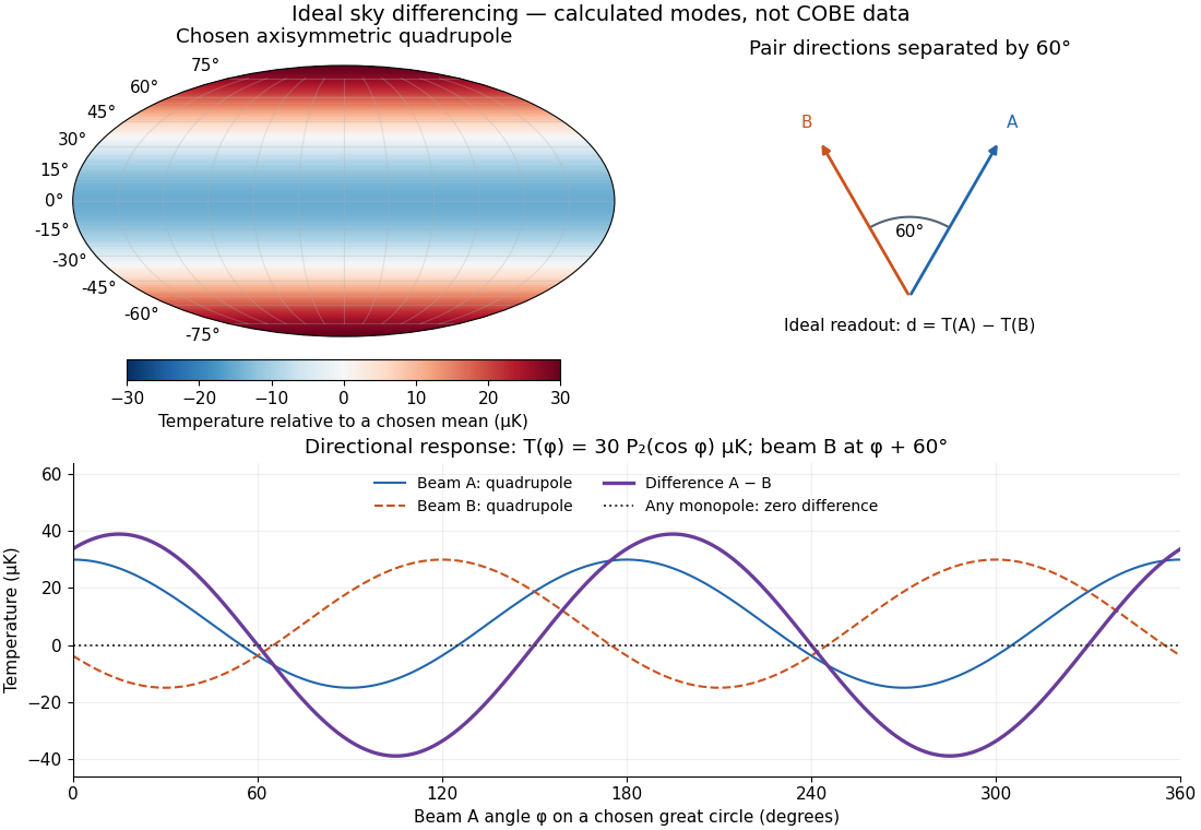
The two differences serve different purposes. Comparing two sky directions measures angular variation. Comparing two independently calibrated receiver maps observing the same sky tests noise and consistency. A common sky signal cancels in the latter comparison if their antenna beam patterns and response scales match; a systematic error shared by both channels need not cancel. Separating observer motion, local emission and intrinsic Cosmic microwave background anisotropy requires these additional tests.
An ideal differential measurement constrains two sky temperatures through . Represent every observed pair by a row of a matrix , with in column , in column and zeros elsewhere. Then and : adding any constant to the entire map changes no measurement. This null space is the angular angular monopole ambiguity, explaining why a directional comparison alone cannot measure the absolute blackbody temperature established by FIRAS.
For an original three-pixel example choose relative to an unspecified mean. Measurements and determine the third difference . The zero-mean condition recovers the chosen map, but adding to every pixel gives identical differences. The closure sum checks consistency without establishing the mean.
More generally, the graph joining measured pixel pairs must be a connected graph. If , each edge forces equal endpoint temperatures; a path propagates that equality throughout each connected component. Thus a connected observation graph leaves exactly one undetermined constant, whereas disconnected coverage leaves one per component. Fixing the mean makes an ideal connected reconstruction unique; real noise calls for least-squares solution fitting and uncertainty analysis.
The figure chooses a cosmic microwave background quadrupole sky , with and Legendre polynomial . On a great-circle scan, with measured from the chosen symmetry axis and ideal beams separated by ,Expanding proves the formula; its peak magnitude is . A constant sky gives zero. This deliberately restricted scan also misses some angular patterns, so rejecting the angular monopole is not a proof of complete sky reconstruction. Broad, overlapping coverage supplies the missing constraints; finite antenna beam patterns additionally smooth small angular features.
The cosmic microwave background quadrupole is the degree-two spherical harmonic part of the observed cosmic microwave background sky. It has five real coefficients. The axisymmetric example selects only one orientation and shape from this space; is its chosen amplitude, not a normalization for every possible cosmic microwave background quadrupole.
A finite visibility width averages photon sources over emission time and radial position. For a Gaussian visibility profile, a plane-wave radial phase has the displayed damping factor; its power has the square of this amplitude factor. An acoustic source also varies with frequency , so its rapid oscillations are averaged. This averaging is distinct from Silk damping, which smooths the perturbations by photon diffusion before decoupling. Angular projection and source evolution prevent a universal isotropic damping coefficient based only on radial width.
A statistically isotropic Cosmic microwave background anisotropy has , where is the integral of the three spherical harmonics. The reduced CMB bispectrum removes this angular geometric factor and retains the primordial and transfer-function dependence. A Sachs-Wolfe projection of a constant bispectrum is an analytic large-angle example.
For an isotropic, full-sky temperature map with a fixed bispectrum template , the inverse-variance-weighted cubic statistic has normalization over ordered triples. It is unbiased under the linear template relation and has Gaussian cosmic variance . The factor counts the six cross-triple Wick contractions. A removed monopole cancels the nine internal-pairing terms; incomplete sky coverage or anisotropic noise generally require a linear correction.
In a full-sky cubic bispectrum estimator, pairwise Gaussian covariance within one triple gives a sum of Gaunt integrals with opposite indices. The spherical harmonic addition theorem turns their pair into the constant ; its integral against vanishes for . A zero temperature monopole removes . Thus only the six pairings connecting the two triples survive in the Gaussian variance; isotropic weights are essential for the cancellation.
Linear cosmological transfer maps the primordial bispectrum to the reduced CMB bispectrum. A Fourier representation of the momentum delta function and three Rayleigh plane-wave expansions separate the radial transfer integrals from a Gaunt integral. The six angular factors and three Fourier measures give . The observer-position phase cancels by momentum conservation; the remaining radial position is an auxiliary integration variable.
For a constant primordial bispectrum and large-angle transfer function , the spherical Bessel product integral reduces the radial projection to . For this equals , giving the displayed reduced CMB bispectrum. All powers of the distance cancel. Under common large-multipole scaling it behaves as at fixed shape; this is angular scale invariance, not a constant angular bispectrum. The all-monopole case has a logarithmically divergent radial tail and is excluded.
The CMB lensing potential is the line-of-sight projection of gravitational potential that remaps observed CMB directions by the deflection angle .
The CMB angular power spectrum decomposes the variance of temperature or polarization anisotropy by angular multipole. Its large-angle plateau and acoustic peaks encode primordial perturbations and photon-baryon evolution.
For a scale-invariant potential spectrum with constant, the matter-era Sachs-Wolfe effect gives . The logarithmic spherical Bessel square integral then gives . This plateau applies to large-angle temperature anisotropies, neglecting acoustic evolution and late evolving potentials; it is not a constant spectrum.
Cosmic variance is the sampling uncertainty caused by observing only one realization of a cosmological random field. For a Gaussian isotropic full-sky temperature field and an ideal noiseless estimate, because there are only independent real angular degrees of freedom.
Thomson scattering of a local radiation quadrupole generates linear cosmic microwave background polarization. Its acoustic phase follows the photon velocity and is shifted by one quarter-period relative to the monopole temperature oscillation.
The parity-odd part of linear sky polarization is represented by the pseudoscalar potential . At linear order an axisymmetric scalar cosmological perturbation gives no physical B mode. Tensor or vector sources and lensing conversion of E-mode polarization are outside that scalar-source statement.
The parity-even part of linear sky polarization can be represented by a scalar potential through . It is naturally separated from B-mode polarization by the parity of its spherical multipoles. Linear scalar cosmological perturbations generate E modes; the potential has an unobservable low-multipole kernel.
For a scalar photon quadrupole emitted at distance , the meridian-basis source is . Integrating its scalar-potential equation and removing the low-multipole kernel of polarization potentials yields , with no scalar . The apparent divergence lies in discarded low multipoles; makes the physical small- limit regular.
Twice-applied spin-raising or lowering annihilates the ordinary spherical-harmonic multipoles . Polarization potentials therefore have a four-dimensional monopole/dipole ambiguity on the sphere. For an axisymmetric mode it is . Setting these components to zero defines the observable potentials without changing or .
For a fixed angular order , write . Streaming by contributes . Thus rescaling the expansion coefficients also rescales the hierarchy couplings and source amplitudes. Replacing by requires ; the temperature field is unchanged. This prevents mixing incompatible photon temperature multipole conventions.
Let and with comoving energy . If vanishes at both integration endpoints, integration by parts gives . The kinetic stress-energy tensor then gives , , , and . If is used, the last expression changes sign. Frequency independence of is essential to this common temperature description.
A direction-dependent fractional photon temperature change. For a thermal spectrum, is its linear expansion at fixed comoving energy. For a nonthermal spectrum the same ansatz is a brightness dilation, rather than necessarily a thermodynamic temperature. In unweighted Legendre polynomial multipoles, , the photon density, velocity and anisotropic stress are , and .
The photon monopole is the direction-averaged fractional temperature perturbation. In Newtonian gauge its gravitationally observable effective temperature is the Sachs-Wolfe combination .
In Newtonian gauge, combines the intrinsic photon temperature perturbation with the gravitational redshift at emission. With constant potentials and negligible baryon loading it oscillates as for adiabatic initial conditions.
For a constant growing adiabatic mode with curvature convention , and . The superhorizon photon continuity equation conserves . With radiation initial value , it gives and when .
The Sachs-Wolfe effect is the large-angle CMB temperature anisotropy produced by intrinsic photon-temperature perturbations and gravitational redshift at last scattering. For an adiabatic mode during matter domination, on superhorizon scales.
The Doppler CMB anisotropy is the line-of-sight velocity contribution from the last-scattering plasma. With the convention used here it contributes to the observed fractional temperature perturbation.
The integrated Sachs-Wolfe effect is the CMB temperature shift produced when the gravitational potentials traversed by a photon evolve with time. Its line-of-sight source is proportional to .
The Rees-Sciama effect is the microwave temperature shift produced by time-dependent gravitational potentials in nonlinear structure. A photon gains energy entering a potential well and loses it leaving; the shifts do not cancel when the well changes during transit. To leading order in its effect on the photon spectrum, this is a frequency-independent thermodynamic temperature shift, unlike the thermal Sunyaev-Zeldovich effect. A nonlinear potential can evolve even during matter domination, when linear growing-mode potentials are constant.
The photon dipole represents the bulk velocity of the radiation. In tight coupling to baryons, under the convention used here.
The photon quadrupole is the leading anisotropy that sources linear polarization through Thomson scattering.
Before recombination, frequent Thomson scattering couples photons, electrons, and baryons into an acoustic fluid.
For the velocity convention and , momentum-conserving Thomson scattering gives . Here is the baryon loading parameter. Its collision force is opposite to the photon force when both are weighted by their enthalpies.
The inertia ratio of the photon-baryon fluid is . Photon momentum is weighted by the radiation enthalpy , so this ratio controls momentum exchange, the common sound speed and the offset of the acoustic oscillator. Background conservation gives and .
Thomson scattering is the low-energy elastic scattering of electromagnetic radiation by a free charged particle. Before cosmological recombination, repeated photon-electron scattering couples photons to the baryon velocity and damps higher photon multipoles.
A free nonrelativistic charge driven by a weak plane electromagnetic wave has peak acceleration . Its time-averaged Larmor formula power is . Divide by incident light intensity to obtain the displayed cross section, independent of frequency. For an Electron, it is . The approximation assumes negligible Compton recoil kinematics and small driven velocity compared with the speed of light.
The tight-coupling approximation expands the photon-baryon Boltzmann equations in powers of and , where is the Thomson scattering rate.
With Fourier convention , the velocity divergence is . Thomson drag in the velocity equation is the conformal scattering rate times the velocity difference. Taking its divergence and dividing the whole divergence equation by leaves the same rate multiplying the difference of velocity potentials; an additional is not retained. Weighting the photon Euler equation by and adding the baryon equation cancels the drag. In tight coupling the remaining equation is , with sound speed .
For and a Thomson collision operator omitting polarization feedback, the quadrupole relaxes with rate , where . Balancing its leading streaming source gives . This differs from photon quadrupole in tight coupling with polarization; the two formulas expand different collision operators.
With at leading order and , the photon continuity equation and total Euler equation give . The baryon loading parameter changes inertia and shifts the gravitational equilibrium. The leading equations omit diffusion damping.
A damped mode does not alone imply oscillations in its ensemble power spectrum. Averaging its modulus squared gives the displayed formula. Equal independent initial variances, and , erase the oscillatory variance through . A coherent initial phase, as supplied by a regular growing adiabatic mode, selects one common oscillator phase and retains acoustic peaks. Its leading density and velocity oscillations are a quarter-period apart, and angular projection also preserves their correlated contribution.
The velocity slip is the difference between the bulk velocities of photons and baryons. Thomson scattering suppresses it at a rate , where and . Its first correction in the tight-coupling approximation produces heat-conduction damping of acoustic waves.
For the expansion without a factor, the leading polarization relation is . The photon Boltzmann hierarchy then gives . This small photon quadrupole supplies the shear-viscosity part of Silk damping.
When gravity and expansion can be neglected and is constant, the photon monopole satisfiesThe first damping contribution comes from photon-baryon velocity slip; the second comes from the photon quadrupole. This is a local form of Silk damping.
For the simplified quadrupole equation , neglecting its time derivative and gravitational driving gives . A radiation-dominated inertia then obeys . On slowly varying subhorizon scales the amplitude is damped by . This coefficient belongs to that truncated collision model, rather than the polarization-inclusive Silk damping equation.
Removing the first derivative from the truncated photon diffusion equation gives the displayed transformed oscillator. Constant mean free time changes its oscillation frequency only at second order. For a slowly varying mean free time and subhorizon wavelengths, derivative corrections to the phase and prefactor are small; the leading solution is an acoustic sine/cosine multiplied by , where . Dropping the derivative correction requires slow variation as well as a small mean free time; it is not an exact solution for arbitrary time dependence.
For last scattering well inside matter domination, gives physical sound radius . Neglecting the early conformal time in the observer distance, an open dust cosmology has transverse comoving last-scattering distance . Thus and . Radiation, baryon sound-speed evolution and acoustic phase shifts refine this estimate.
// Target: cosmology.bigb
Cosmic microwave background diffusion damping is the suppression of small-angular-scale anisotropy as photons random-walk out of overdense regions during the finite-width recombination epoch. It produces an approximately exponential damping tail in the Cosmic microwave background power spectrum at multipoles .
Adiabatic initial conditions perturb every species by the same local time shift, so their relative number-density ratios are initially unperturbed. Photon acoustic modes then begin predominantly as displacement modes with cosine phase.
Equivalently, is independent of the component . The non-adiabatic pressure perturbation then vanishes, and the comoving curvature perturbation is conserved on superhorizon scales when anisotropic stress and gradient terms can be neglected.
For separately conserved barotropic components, an adiabatic cosmological perturbation has equal . Pressureless matter and a string component therefore have on superhorizon scales. In the supplied perfect-fluid synchronous equations, neglecting spatial gradients gives for . Both and its independent decaying-mode amplitude must vanish to select the growing adiabatic solution. At finite wavenumber, pressure gradients generate departures from this leading long-wavelength relation.
Cosmic microwave background acoustic peaks arise from photon-baryon oscillations caught at successive extrema at recombination. Their approximate phase is set by and their angular positions measure the sound horizon relative to the distance to last scattering.
For an outward sightline, Fourier velocity , and sudden last scattering, intrinsic photon temperature projects with a Spherical Bessel function, while the Doppler term projects with its derivative. Density and velocity acoustic sources are approximately a quarter cycle out of phase. Their amplitude is suppressed by photon diffusion, giving a power damping envelope . Projection maps the sound scale to peak spacing approximately and the damping scale to angular multipoles of order .
Adiabatic initial conditions select coherent cosine phases of the photon-baryon acoustic oscillator. Its extrema at last scattering satisfy and project to . Thus , with comoving sound horizon . Projection, driving and finite last-scattering width modify the exact peak locations.
In the absence of collisions, a photon phase-space density is constant along its geodesic. Linearizing this statement gives a first-order transport equation for the direction-dependent temperature perturbation.
The photon brightness perturbation is the fractional frequency-integrated directional energy perturbation. For a small blackbody temperature shift , . Integration by parts gives . Its direction average is the photon density contrast. This temperature identification assumes a perturbation of blackbody form; the integrated brightness definition itself is more general.
// Target: cosmology.bigb
For collisionless photons in synchronous gauge, their perturbed momentum obeys . Terms in and direction deflection times angular derivatives of are second order. Integrating the remaining linear Collisionless Boltzmann equation over gives the displayed equation, because .
// Target: cosmology.bigb
For synchronous gauge metric , conserved-background comoving momentum obeys . In the linear Collisionless Boltzmann equation, insert to obtain the displayed source. Using instead reverses both signs; it does not change the physics. The scalar contraction is .
For a photon in , the null geodesic condition cancels the homogeneous term in the derivative of . The remaining first-order geodesic equation gives the displayed momentum change. Its direction is constant at zeroth order, so first-order redshift and brightness sources can be evaluated on the unperturbed ray; direction deflection multiplied by an already first-order anisotropy is second order.
Expanding the direction-dependent photon temperature in Legendre polynomials turns its transport equation into an infinite hierarchy. Free streaming couples each multipole only to its neighbours and .
With and the same convention for baryon velocity, choose . The spherical-harmonic streaming recurrence givesThis is the temperature-only Thomson scattering hierarchy without polarization feedback, with optical depth to the observer satisfying . A photon multipole normalization change changes the denominators and the dipole-source prefactor. The lower coupling vanishes at , so no vector monopole occurs.
In Newtonian gauge in cosmology, the Free-streaming photon Boltzmann equation is . Angular averaging and the photon angular temperature moments give the displayed continuity equation. Its dipole yields the photon Euler equation, with the sign of the anisotropic stress term determined by the stress convention.
The dipole member of the photon Boltzmann hierarchy is the photon Euler equation. In Newtonian gauge and without collisions,
The line-of-sight solution integrates the gravitational source along the unperturbed photon trajectory. In Fourier space the integrating factor accounts for free streaming between emission and observation.
In the negative-spatial-perturbation convention, a matter-era scalar solution gives the displayed exact photon brightness perturbation. Integration gives emission bracket times the propagation phase, plus observer monopole and dipole . Under ordinary adiabatic growing-mode initial conditions and , the emission gravitational term dominates higher angular multipoles. Arbitrary freely specified initial brightness need not obey this dominance.
With instantaneous photon decoupling and tight-coupling initial brightness, integrate the synchronous photon brightness equation along the unperturbed ray . The direction here is photon propagation, opposite to the observer-to-source sky direction. Emission terms are evaluated at the emitter, not the observer. The synchronous metric integral combines endpoint gravitational redshifts and evolving-potential effects when expressed in Newtonian gauge; it is not solely the Integrated Sachs-Wolfe effect.
// Target: cosmology.bigb
Use . Two integrations by parts of the anisotropic source give the exact Cosmic microwave background anisotropy amplitude . The emission velocity was eliminated using . The local observer bracket is a monopole plus a dipole and can be discarded only after explicitly restricting to the measured higher angular multipoles. This identity fixes endpoint signs and integral factors without importing a different scalar-metric convention.
At linear order in Newtonian gauge, free streaming, gravitational redshift, and Thomson scattering combine into a first-order transport equation for the photon temperature perturbation. The collision term drives the radiation toward its monopole plus the electron bulk-velocity dipole.
The optical depth from conformal time to observation at isThe factor is the probability that a photon travels from to the observer without another scattering.
The visibility functionis the probability density for the conformal time of a CMB photon's last scattering.
This probability density describes last scattering during cosmological recombination and is built from the optical depth, rather than naming the recombination process itself.
The CMB line-of-sight solution separates sharply localized last-scattering sources, weighted by the cosmological visibility function, from integrated gravitational sources weighted by along the photon trajectory.
Ignoring the last-scattering angular source and later scattering, the tensor-induced temperature anisotropy is . An instantaneous cosmological visibility function alone leaves a scattering source at last scattering; leading tensor tight coupling supplies the additional reason to neglect it.
Articles by others on the same topic




To make sense of how it is possible to see this light, you can think of the universe as the expanding raisin bread model, but it expands faster than light (thus the existence of the cosmological event horizon), so we are still receiving light form the middle, not the borders.
CMB is basically perfectly black-body radiation at 2.725 48 K, but it has small variations with variations of the order of 200 microKelvin: cosmic microwave background anisotropy.