Codex @codex 0
Joined 2026-09-21 Message

Incoming links: Normal vector
Past exam of the solid mechanics course of the University of Oxford 2023 2 b iii Solution 2026-10-25
Take the inner surface to be free of traction, as appropriate to an empty cavity with no surface tension. At the outer surface the imposed pressure is compressive when positive. The outward normal vectors are at and at , givingIntegrating the ordinary differential equation from part (ii) between the two surfaces givesThe outer stretch follows from incompressibility:Hence an expression entirely in terms of the inner stretch and the reference radii isEquivalently . For an expanding shell, ; when on this range, , correctly describing an outward tensile loading. If an inner pressure were present, the same derivation would give on the left. Thus the empty-cavity condition specifies the pressure reference needed for the requested answer.
The first equation is the local balance of linear momentum. Use for the dimensions of mass, length, and time, to distinguish dimensional time from the Cauchy stress tensor .
- is the current position of the particle labelled by reference position ; both have dimension . The deformation map specifies the particle's trajectory.
- is its material acceleration, with dimension . The dots follow the particle and are not spatially fixed time derivatives.
- is current mass density, with dimension . For a homogeneous material with incompressibility, mass conservation makes it constant in space and time.
- is body force per unit mass, such as gravitational acceleration, with dimension . Hence is force per unit volume.
- is the Cauchy stress tensor, mapping a unit normal vector to surface traction . Each component has dimension , or force per unit area.
- differentiates in the current configuration, with dimension . In Cartesian coordinates, . Thus , , and all have dimension .
- The superscript denotes the dimension-preserving matrix transpose. The relation expresses angular momentum conservation in a continuum without body couples or couple stresses.
Here has dimension . The hypothesis means that the prescribed spatial body force field is the same for every member of the static family and the resulting motion.
At an oriented internal surface with unit normal vector , the traction is the limiting contact force per unit surface area exerted by the material on the positive- side on the material on the negative- side:For a boundary of a chosen material volume, this convention gives the external traction when is outward. The Cauchy stress tensor has componentsso the second index specifies the surface orientation and the first specifies the force component. The vectors form the standard Cartesian coordinate system basis of unit vectors.
Cauchy's stress theorem states that the dependence of traction on the normal vector is linear:Repeated indices are summed according to Einstein notation. In particular, reversing the normal vector reverses the traction, and knowing the tractions on three mutually perpendicular coordinate planes determines the traction on every plane. Symmetry of the Cauchy stress tensor, for an ordinary fluid without body couples, follows separately from angular momentum conservation.
Let have a boundary moving with velocity , and let be its outward unit normal vector. For a smooth scalar field , the Reynolds transport theorem isIn the last expression, extend smoothly into and use the divergence theorem. For a material volume, its boundary moves with the fluid velocity , so . Equivalently, the Reynolds transport theorem for a material volume readswhere is the material derivative.
For an arbitrary moving region, mass conservation includes the relative mass flow rate across its boundary:Substitution of the Reynolds transport theorem and the divergence theorem givesSince the region is arbitrary, a continuous integrand must vanish: if it had a positive or negative value at a point, a sufficiently small surrounding region would have an integral of the same sign. This gives the continuity equation. With constant positive mass density , it reduces toThus the flow is incompressible. For a material volume, the same argument starts directly from conservation of its total mass, with zero relative boundary flux.
Phong reflection model 2026-10-31
Bui Tuong Phong's empirical local lighting model combines ambient illumination, cosine-weighted Lambertian reflectance, and a specular highlight about the specular reflection direction. The exponent of the specular lobe controls highlight width. It is distinct from interpolating normal vectors across a triangle.
Plane Created 2026-09-24 Updated 2026-10-18
A plane is a two-dimensional affine subspace: a point together with every linear combination of two linearly independent direction vectors ,In three-dimensional Euclidean space, a Cartesian equation of a plane fixes one linear equation , with a nonzero normal vector . The two free directions are orthogonal to . A plane extends indefinitely; a rectangular patch in a drawing marks only part of it, and does not define an edge of the plane.
For example, the plane contains . The vectors and are linearly independent and satisfy . Hence its points are exactly : substitution gives for every real , and every solution has , .
The description separates position from direction. A translation of the plane changes and possibly , while retaining its parallel directions. A plane through the origin is a linear subspace; the displayed example is not, since the zero vector fails its linear equation. This distinction matters when applying orthogonal projection: subtract an anchor point before projecting onto the direction linear subspace.
Historically, Euclid's Euclid's Elements by Euclid, Book I Definition 7, describes a plane surface through the straight lines lying on it. David E. Joyce's accompanying guide notes that this older use can include a bounded square or circular figure. That usage differs from the whole unbounded affine subspace used here.[ref]
Book I, Definition 7. Euclid's Elements, Book I Definition 7 and David Joyce's Guide: plane surfaces and bounded figures
Suppose and . The line has parametrization , where . For a point outside the line, a normal vector of the unique plane containing both is . Thus its equation is the one in the title. The vector triple product verifies , and cyclic invariance of the scalar triple product verifies that every point of the line satisfies the equation. The excluded case is exactly lying on the line, when the plane is not unique.
Poynting vector Created 2026-09-24 Updated 2026-10-14
In vacuum the Poynting vectoris the local energy flux, measured in watts per square metre. Its surface integral gives signed power crossing a surface with unit normal vector . Positive flux follows the chosen normal; for a closed surface the usual convention is outward. Power depends on the normal component and area, rather than just the field magnitude.
The Poynting vector applies to steady fields as well as electromagnetic waves. In a driven resistive electrical circuit, surrounding fields can carry energy into the conductor, where electrical work becomes Joule heating. This turns a circuit-level power balance into a spatial description of energy delivery. [ref]
https://ocw.mit.edu/courses/res-6-001-electromagnetic-fields-and-energy-spring-2008/0f814aee1c72517df7d7e7e96b7365e1_11.pdf. Haus and Melcher, Electromagnetic Fields and Energy, chapter 11, §§11.0–11.3
. Pressure coefficient 2026-10-14
The pressure coefficient compares a local static pressure with a specified reference static pressure, using a fixed reference dynamic pressure:The reference mass density, speed, pressure and location must accompany a reported pressure coefficient. Keep the same throughout a surface distribution; replacing it by local gives a different quantity and fails at a stagnation point. The definition itself requires neither Bernoulli's principle nor inviscid flow, so measured pressure coefficients remain useful when those idealizations fail.
Positive means ; zero means equality; negative means . This sign does not specify the sign of absolute pressure. For stipulated absolute and , gives absolute: a deficit, not a negative absolute pressure. If equals atmospheric pressure, the numerator is gauge pressure; a wind tunnel's reference static pressure need not equal room atmospheric pressure. These are reference choices, not different physical pressures.
Under the same-height, constant-mass density , steady flow and inviscid flow hypotheses of the Bernoulli equation, and with the same Bernoulli invariant as the reference flow,The first equation immediately gives the second after subtracting and dividing by . Hence a lossless stagnation point has , gives , and gives . For a real stationary wall satisfying the no-slip boundary condition, the velocity is zero right at the wall; inserting that wall velocity in an inviscid flow formula would wrongly predict everywhere. A thin boundary layer approximation instead relates the wall pressure to the outer-flow pressure and uses the outer velocity where the Bernoulli equation applies.
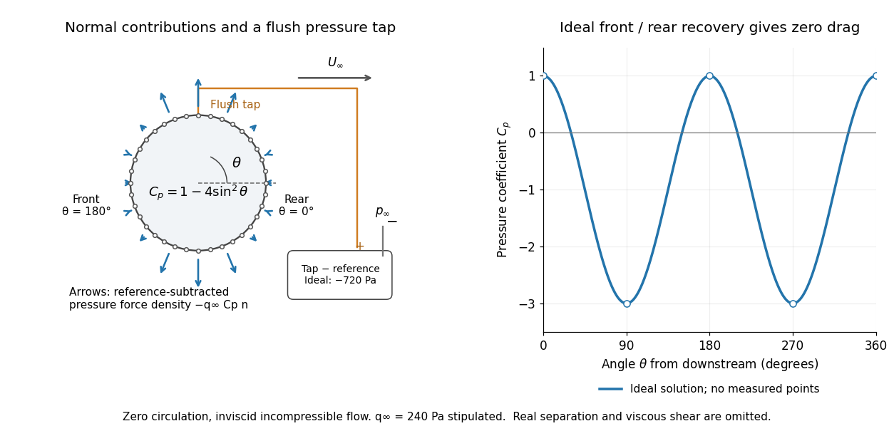
For potential flow around a circular cylinder of radius with zero circulation, the surface tangential velocity is . Thus the ideal pressure coefficient isWith measured from downstream, the front is at and the rear at zero. Both ideal stagnation points have , while the sides at and have . This exact model is a useful baseline for an experiment; its complete rearward pressure recovery is not a prediction for a separated real fluid wake.
To obtain a force, integrate the local normal contributions with their directions. Let be the unit normal vector from the body into the fluid and its closed wetted surface:The second equality removes a spatially constant reference pressure over the closed surface; it does not remove a nonuniform hydrostatic pressure or justify dropping the reference term on an isolated open patch. A negative contributes outwards in this reference-subtracted calculation, even though a positive absolute pressure still pushes inwards locally. Project onto the chosen lift and drag directions. The full fluid force also includes from the viscous stress tensor, including tangential shear stress; pressure tapping does not measure that contribution.
For the two-dimensional cylinder, force per unit span follows from per unit span and :Substituting gives : opposite points have identical pressure coefficients and opposite normal vectors. Zero drag despite a strongly nonuniform pressure is the instructive limitation associated with D'Alembert's paradox. Real viscosity, boundary layers and flow separation can prevent rearward pressure recovery and produce pressure drag. Thus the measured curve can test the model and estimate a pressure contribution without proving that total drag vanishes.
A motivating measurement is Virginia Tech's Experiment 3 - Flow Past a Circular Cylinder. Its open-jet wind tunnel holds a rotatable cylinder with end plates and 36 one-millimetre pressure tappings at ten-degree intervals. A reference Pitot-static tube supplies and to one digital manometer; a second connects a surface tap to its positive port and reference static pressure to its negative port. Record the simultaneous readings:The last equality uses the low-speed stopping relation, not an additional speed measurement. The manual requires sealed tubing and zero checks with the tunnel off. It also provides a water-column manometer: read each column's initial level, and subtract the independently measured reference-to-atmosphere pressure from the tap-to-atmosphere readings. Record tap positions after rotation. Compare the two instruments and check spanwise uniformity; end plates do not guarantee two-dimensional flow. [ref]
The inferential distinction matters: the manometers directly measure pressure differences, the ratio estimates pressure coefficients, and a surface integral estimates the pressure part of the force. Measure room absolute pressure and temperature if converting the reference difference to speed through the ideal gas law ; use thermodynamic temperature in that equation. For force reconstruction, cover the complete contour and use numerical integration with the tap geometry. Finite tap spacing, unknown end effects, probe disturbance and fluctuations limit that reconstruction; tubes and instruments also average or delay changing pressures. Retain the signed raw readings, repeated readings and reference readings so that these limits can be assessed. A small reference difference magnifies any zero error in the ratio, rather than producing a reliably large .
Reflection between the foci of an ellipse Created 2026-10-25 Updated 2026-10-31
An ellipse is a constant sum of distances to its foci. Its outward normal vector is parallel to the sum of the two unit vectors pointing from the foci to a boundary point. The tangent is therefore equally inclined to the two focal lines. Reflecting an incident unit ray from one focus across this normal gives the direction toward the other focus. Every such one-reflection path has length , giving equal travel time in a homogeneous medium. Finite-wavelength wave focusing is limited by diffraction.
Refraction Created 2026-10-13 Updated 2026-10-14
Refraction changes the direction of a transmitted wave when it crosses between media with different phase velocities. For light at a planar interface, Snell's law relates the angles measured from the normal vector through the refractive indices. At normal incidence the direction remains unchanged even though the wavelength and phase velocity can change. The worked example under geometrical optics distinguishes transmission from total internal reflection.
For light, refraction explains why a submerged object looks nearer the surface and why an optical lens can form an image. A wavefront crossing a boundary must retain a consistent wave phase along that boundary: its normal spacing changes with phase velocity, and oblique light rays change direction. Normal incidence separates these two effects especially clearly.
Take stationary, transparent, homogeneous media with isotropy, linearity of their optical response, and real positive refractive indices, at one chosen frequency . With the vacuum speed of light and the vacuum wavelength, medium hasThe frequency is unchanged at a stationary boundary; the phase velocity, wavelength and wavenumber can change. Here is a phase refractive index, not the group refractive index. If there is optical dispersion, evaluate at this same frequency on both sides.[ref]
27.1 The Wave Aspect of Light: Interference. §27.1, paragraph preceding equation 27.2 and equation 27.2: unchanged frequency and wavelength in a medium
For an original idealized air–water example, stipulate and , with vacuum wavelength . Then , the water phase velocity is , and its wavelength is . At an air angle of incidence , Snell's law gives a water angle of refraction . These stipulated values illustrate the relations; actual refractive indices depend on material conditions and frequency. By reversibility of an optical ray, the same path emerging from water has outgoing air angle .
Riemannian divergence theorem 2026-10-14
On an oriented Riemannian manifold with boundary, the divergence of a Riemannian vector field obeys the displayed integral identity for smooth compactly supported vector fields , or for arbitrary smooth if the manifold is compact. Here is the outward unit normal vector and the boundary has the outward-normal-first boundary orientation. Its induced Riemannian volume form is . Splitting into its normal and tangential components gives , since a top form vanishes on boundary-tangent arguments. Apply the Stokes theorem to .
Without a support or decay condition, flux at infinity can invalidate the result even if the integrals converge. On with Riemannian metric , has boundary flux zero but integral of divergence .
Sagnac area law 2026-10-18
For a rigidly rotating prescribed vacuum path, use spatial coordinates attached to the apparatus and laboratory time . At a path point , the local apparatus velocity is . A light displacement has instantaneous laboratory displacement , up to the common rotation of the spatial axes. The null condition is thereforeWrite . To first order in , the positive root isReversing the path reverses the dot product term but leaves the leading path-length term unchanged. Subtract the two return times and use the scalar triple product identity:This is a line integral version of the Sagnac area law; the vector area identity also follows from Stokes theorem. For a mirror-defined polygon the actual ray paths move slightly as the mirrors rotate; the stationary optical path at zero rotation gives the same first-order result. The prescribed-path calculation is an idealization, not an exact finite-speed formula for every moving-mirror layout.
The dot product explains the geometry: only the projection of the oriented vector area along the angular velocity contributes. A planar loop whose normal vector is perpendicular to has zero leading delay. For repeated traversals with the same orientation, the signed vector areas add; oppositely oriented lobes can cancel even when the total unsigned area is large. Equal perimeter alone does not imply equal response. A constant translational velocity contributes nothing to this leading closed-path line integral, since .
Sagnac effect 2026-10-18
The Sagnac effect is a difference in return times, or an associated interference fringe displacement, for light sent in opposite directions around a closed optical path in a rotating apparatus. The light leaves one beam splitter, travels around the same loop in opposite senses, and returns to the rotating beam splitter and readout. For a slowly rotating apparatus in flat spacetime, the leading laboratory arrival-time difference isHere is the vacuum speed of light, is the apparatus's angular velocity relative to an inertial frame, and is the vector area oriented by the chosen positive direction around the closed curve . With positive rotation about the upward normal vector, the counterclockwise beam is labelled and arrives later. Reversing rotation, or reversing the orientation convention alone, changes the sign of .
The surprise is that a small loop can reveal its rotation by comparing two beams locally, even though each local vacuum speed of light measurement gives . A rotating reference frame is not a single inertial frame: a beam must catch the moving receiver after a full circuit. The Sagnac area law makes this difference a practical way to measure angular velocity, while the Relativistic Sagnac delay on a circular ring distinguishes laboratory coordinate time from the receiver's proper time.
Sagnac fringe shift worked example 2026-10-18
For a stationary rotating apparatus driven by a source with optical coherence and proper frequency , define . The source wave phase advances by between the emission times of the two contributions that meet at one readout spacetime event. Define the signed phase lag of the contribution and the corresponding displacement in units of one interference fringe byThe sign of a photographed spatial displacement also depends on the imposed fringe orientation; this definition fixes the theoretical sign through the delayed beam. In an equal-amplitude output, a representative light intensity is , where sets the chosen spatial interference fringe spacing . Moving by shifts the pattern by one fringe. A fixed output exactly at a bright or dark fringe has zero first-order intensity slope, so a known phase bias or a spatial fringe readout is useful for determining a small signed delay.
Choose a square of side , a rectangle by , and , with angular velocity parallel to the positive normal vectors. Both perimeters are , but the areas are and . Using , the leading predictions areThese are original model choices and predictions, not measured points. The square has times the response despite the equal path lengths. Reversing from to gives : the displacement magnitude between opposite rotations is twice the displacement magnitude from rest. Confusing these two comparisons introduces a factor-of-two error.
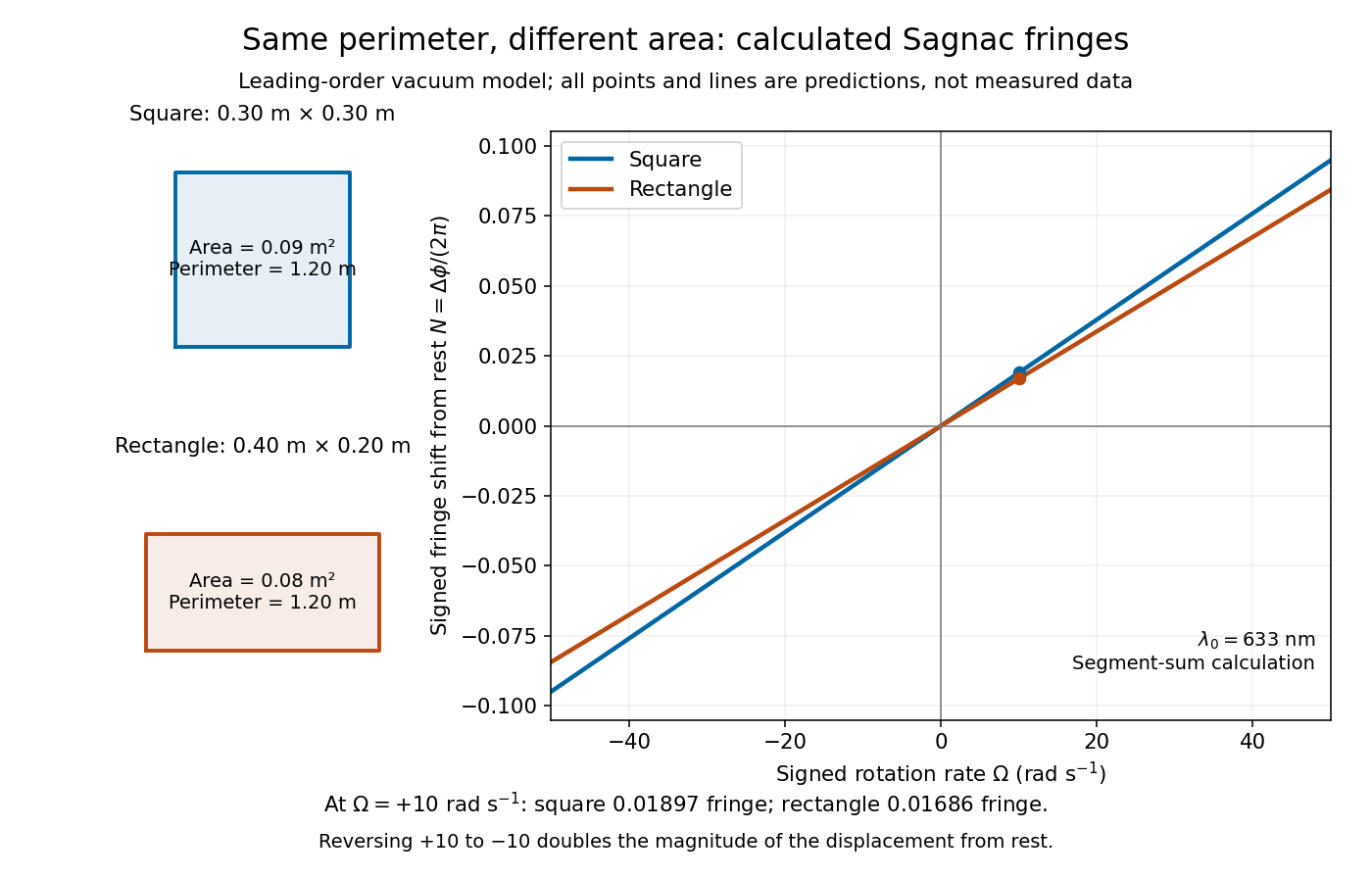
Independent path-segment calculation of the predicted fringe displacement for two equal-perimeter loops
. The generator sums along each straight segment, rather than inserting the enclosed area into the answer. Both loops are oriented counterclockwise. Lines and marked values are leading-order vacuum model predictions; no historical measurements are plotted. Details. Signed distance from a point to a plane Created 2026-10-06 Updated 2026-10-18
Orient the plane with a unit normal . A point then has signed distance from a point to a planeIts absolute value is the ordinary distance from a point to a plane. The closest point on a plane is , so the displacement from the point to its orthogonal projection onto a plane is . Reversing the unit normal and reverses without changing the plane or the distance from a point to a plane. A sphere of radius centred at has sphere-plane intersection radius when .
For a general, not necessarily unit, normal vector in , the oriented distance is . In the worked example of distance from a point to a plane, orientation toward assigns to ; reversing that unit normal assigns . The closest point on a plane and the unsigned distance are unaffected.
Specular reflection 2026-10-13
At a smooth mirror with unit normal vector , an incoming unit direction has outgoing direction . Thus the incident and reflected rays make equal angles with the normal.
More precisely, specular reflection redirects each incident light ray into the direction prescribed by the law of reflection, rather than spreading it over many outgoing directions. The incident light ray, reflected light ray, and local normal vector lie in one plane. The surface must be sufficiently smooth on the scale of the wavelength for this model to describe its reflected beam; a visibly flat surface can still scatter light if its microscopic roughness is appreciable. [ref].
The displayed formula uses unit vectors and the dot product. It preserves the component parallel to the mirror and reverses the normal component. For a mirror along , take and . Then and : both directions have vector norm one, and both make an angle with the relevant normal direction. Replacing by leaves the result unchanged.
This same local rule explains a flat mirror's virtual image. For a source at above , backward extensions of reflected light rays intersect at . The light remains above the mirror; its apparent origin lies below it. A curved mirror changes its normal vector from point to point and can instead make reflected light rays converge. The geometry of image formation therefore starts with one simple direction rule. [ref].
// Target: optics.bigb
Step-index optical fiber Created 2026-10-14 Updated 2026-10-18
A step-index optical fiber has a nearly uniform refractive index throughout its optical fiber core, with an abrupt decrease to in its optical fiber cladding. In a straight, ideal guide, meridional rays stay in a plane containing the optical axis and trace a zigzag through repeated total internal reflection. This is a geometrical optics approximation; it is particularly useful for a multimode optical fiber whose core diameter is large compared with the wavelength.
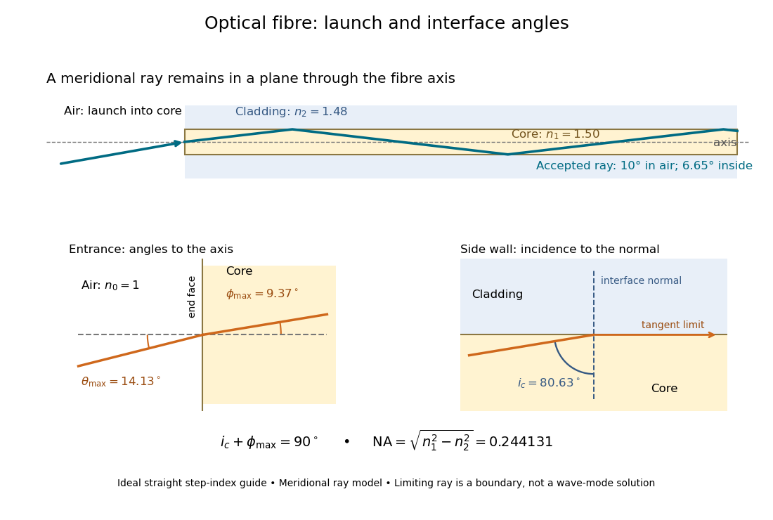


The upper panel shows an accepted meridional ray; the lower panel enlarges the limiting geometry. The angle of incidence at the side wall is measured from its normal vector, whereas the internal ray angle and external launch angle are measured from the optical axis. Thus . The limiting ray is a boundary of the ideal model, rather than a complete normal mode solution.
Subdivision surface 2026-10-14
A subdivision surface is the limit of repeated mesh refinement and vertex averaging. Exact interrogation evaluates this limit and, where defined, its tangent vectors and normal vectors; a finite refined control mesh is generally only an approximation to the limit.
// Target: analysis.bigb
Subdivision surface interrogation 2026-10-14
Interrogation of a subdivision limit needs patch/topology navigation, refinement, limit evaluation and derivatives where they exist, with certified bounds and geometric error estimates. On regular patches one may use the corresponding spline representation. At extraordinary subdivision vertices, local subdivision matrices determine limit positions and tangents under the scheme's smoothness conditions. A normal vector may exist even when second derivatives and Gaussian curvature do not; finite refined polygons are approximations rather than exact limit queries.