Past exam of the mathematics course of the University of Cambridge / 2013 / ib / Paper 2

Write $U^{\ast }={\overline{U}}^T$ for the conjugate transpose. Taking determinants in $U^{\ast }AU=A$ gives $|\det U{|}^2\det A=\det A$. Since the Hermitian matrix $A$ is invertible, every such $U$ is invertible and $|\det U|=1$. The identity belongs to $U_A$; if $U,V\in U_A$, then $(UV{)}^{\ast }A(UV)=V^{\ast }AV=A$; and multiplying $U^{\ast }AU=A$ by $(U^{\ast }{)}^{-1}$ and $U^{-1}$ gives $(U^{-1}{)}^{\ast }A{U}^{-1}=A$. Associativity comes from matrix multiplication, so this is a group.

The Hermitian form $h_A(v,w)=v^{\ast }Aw$ obeys $h_A(Uv,Uw)=h_A(v,w)$ precisely when $U\in U_A$. Thus $U_A$ is the group of linear isometries of this nondegenerate Hermitian form; positivity of $A$ is unnecessary.

For $A=I$, $U$ is a unitary matrix. Here is a direct diagonalization of a matrix proof. Over $\mathbb{C}$, its characteristic polynomial has a root, giving a unit eigenvector $v$ with $Uv=\lambda v$. Preservation of the inner product gives $|\lambda |=1$. If $w\perp v$, then $⟨Uw,Uv⟩=⟨w,v⟩=0$, so $v^{\perp }$ is invariant. The restriction is again a unitary matrix. Induction on the dimension supplies an orthonormal basis of eigenvectors. In that basis, $U$ is diagonal, with diagonal entries on the unit circle.

Let $R$ be a Euclidean domain and $I$ a nonzero ideal. Choose $d\in I\setminus \{0\}$ minimizing the Euclidean size. For any $a\in I$, Euclidean division gives $a=qd+r$, where either $r=0$ or $r$ has smaller size than $d$. But $r=a-qd\in I$, so minimality forces $r=0$. Consequently $I=(d)$. The zero ideal is $(0)$, proving that every Euclidean domain is a principal ideal domain.

A commutative ring is Noetherian if every ideal is finitely generated; equivalently, every ascending chain of ideals stabilizes. To see the equivalence, the union of an ascending chain is an ideal. Finitely many generators for that union already belong to one member of the chain, after which the chain is constant. Conversely, an ideal which is not finitely generated permits successive choices outside the ideals generated by previous choices, producing a strictly ascending chain.

Every principal ideal domain is therefore Noetherian. The given Euclidean domain property of the Gaussian integers yields

Both maxima exist by continuity on the compact set $[a,b]$. Their sum is nonnegative and vanishes only for $f=0$. The identities $\Vert cf{\Vert }_1=|c|\Vert f{\Vert }_1$ and the triangle inequality follow by applying the corresponding supremum norm facts to $f$ and $f^{\prime }$. This proves that $\Vert \cdot {\Vert }_1$ is a norm.

For $m=(a+b)/2$, $|\Phi (f)|=|f^{\prime }(m)|\le \max |f^{\prime }|\le \Vert f{\Vert }_1$. Hence the first unit ball has image contained in $[-1,1]$: derivative evaluation is a bounded linear functional for this norm.

For the supremum norm alone, take $f_N(x)=\sin (N(x-m))$. These smooth functions satisfy $\Vert f_N{\Vert }_0\le 1$, but $\Phi (f_N)=N$. Thus the second image is unbounded. The distinction is the unboundedness of derivative evaluation in the supremum norm, not a failure of differentiability of the individual functions.

True. In a discrete topology, the singletons form an open cover. If $X$ is compact, a finite subcover exists, so $X$ is finite. Conversely, any open cover of a finite set has a finite subcover: choose one member containing each point. This converse does not require the discrete topology.

False without a separation assumption. Give $X=\{0,1\}$ the indiscrete topology $\{\varnothing ,X\}$, and take $Y=\{0\}$. Both spaces are finite and hence compact, but $Y$ is not a closed set because $X\setminus Y=\{1\}$ is not open. In a Hausdorff space, a compact subset would be closed; that hypothesis is absent here.

Parametrize the characteristics by $s$, starting from $(x,y,u)=(1,r,r)$. Their ordinary differential equations areThey give $x=e^s$, $y=e^s(r+s)$ and $u=r+s$. Thus $s=\log x$ and $r=y/x-\log x$, soIndeed, $u_x=-y/x^2$, $u_y=1/x$ give $x{u}_x+(x+y)u_y=1$, and $u(1,y)=y$. The initial line is noncharacteristic, and its characteristics cover the half-plane $x>0$. The data do not determine a solution on $x<0$; a smooth solution through the origin is impossible because the differential equation there would read $0=1$.

Take the divergence of the Ampère-Maxwell equation, $\nabla \times \mathbf{B}={\mu }_0\mathbf{J}+{\mu }_0{ϵ}_0{\partial }_t\mathbf{E}$. Since the divergence of a curl is zero vanishes, and Gauss's law gives $\nabla \cdot \mathbf{E}=\rho /{ϵ}_0$, the result isThis is the charge continuity equation.

At an internal point of a homogeneous Ohmic conductor, Ohm's law gives $\mathbf{J}=\sigma \mathbf{E}$. Since $\sigma$ is constant, the charge continuity equation becomes ${\partial }_t\rho =-(\sigma /{ϵ}_0)\rho$. ThereforeThis is charge relaxation. Here $\rho$ is the total charge appearing in the vacuum form of Gauss's law; in a homogeneous dielectric description of free charge the corresponding constant permittivity replaces ${ϵ}_0$.

For a finite isolated body, charge travels to the surface. The bulk formula applies at internal points, not across the interface where electrical conductivity jumps and surface charge density accumulates. Integrating the charge continuity equation over the body, including its surface charge, gives constant total electric charge because no electric current crosses the external boundary. Bulk decay and conservation of electric charge are therefore compatible.

The free surface is a material surface, so its kinematic boundary condition isWith constant atmospheric pressure $p_a$ and no surface tension, the dynamic boundary condition for an inviscid interface follows from Unsteady Bernoulli equation:Write $\varphi =Ux+\phi$, where $\phi$ and $\eta$ are small. Choose the time-dependent potential gauge so the undisturbed right-hand side is $U^2/2$. Retaining first-order terms, evaluated at $y=0$, givesThe incompressibility condition also gives Laplace's equation for $\phi$.

Set $\Omega =\omega -kU$. Substitution of the specified normal mode into the two linearized boundary conditions yields $-i\Omega a=ikb$ and $\Omega b+ga=0$. Eliminating $b$ gives the dispersion relationThe decay factor $e^{ky}$ in a fluid extending to $y=-\infty$ uses $k>0$. With signed wavenumber the decaying factor is $e^{|k|y}$ and the right-hand side is $g|k|$. The frequency shift is the advection of a deep-water gravity wave by the uniform current.

The Rao-Blackwell theorem says that if $S$ is a sufficient statistic and $\delta$ a finite-variance estimator, then ${\delta }^{\ast }=\mathbb{E}(\delta \mid S)$ is an estimator with the same expectation and no larger variance. Sufficiency ensures the conditional distribution, and hence this formula as a function of the data, does not involve the unknown parameter. The tower property of conditional expectation gives $\mathbb{E}{\delta }^{\ast }=\mathbb{E}\delta$, while the law of total variance givesThis proves the theorem and shows that equality holds exactly when $\delta$ is already determined by $S$, almost surely. In particular, unbiasedness is preserved.

Assume $n\ge 3$. Independence gives $\mathbb{E}\hat{\theta }=p_0{p}_1{p}_2=\theta$, so the proposed indicator is unbiased and has variance $\theta (1-\theta )$. The type counts $S=(n_0,n_1,n_2)$ are a sufficient statistic: conditional on them, every ordering of the labels is equally likely. Consequently,For example, the conditional probability of the ordered first three labels is $(n_0/n)(n_1/(n-1))(n_2/(n-2))$. This is Rao-Blackwellization of a multinomial probability product.

If all three $p_i$ are positive, there is positive probability that all three counts are positive. On such an event the conditional indicator has probability strictly between zero and one, so its conditional variance is positive. Thus $\mathrm{Var}({\theta }^{\ast })<\theta (1-\theta )$ for interior parameter values. If any $p_i=0$, then $\theta =0$ and both estimators have zero variance; the printed strict inequality is impossible at those boundary parameters. The valid unrestricted statement is the non-strict inequality.

An cut of a flow network partitions a flow network into $S,S^c$, with source $A\in S$ and sink $B\notin S$. Its cut capacity is the sum of capacities of arcs directed from $S$ to $S^c$; a minimum cut minimizes this sum.

Use the suggested nodes. Give $A\to a_e$ capacity $1$, each $a_e\to b_v$ capacity $M=m+kn+1$, and each $b_v\to B$ capacity $k$. By the max-flow min-cut theorem, a flow of value $kn$ exists once every cut capacity is at least $kn$.

Consider a cut of a flow network containing no crossing arc of capacity $M$, and let $U$ be the intersections on the sink side. Every street incident to $U$ must also be on that side, or its arc to an endpoint in $U$ would cross the cut of a flow network. Hence at least $d(U)$ source-to-street arcs cross, as do the $n-|U|$ intersection-to-sink arcs from the other intersections. Therefore its cut capacity is at leastA cut of a flow network crossing a capacity-$M$ arc has still larger capacity. The cut of a flow network just before the sink has capacity $kn$, proving the maximum flow value is exactly $kn$.

The integral max-flow theorem supplies an integral maximum flow. Every intersection sends $k$ units to the sink; each street can supply at most one unit, assigned to one endpoint. Orient each assigned street away from its assigned endpoint. Orient unassigned streets arbitrarily. Then each vertex has at least $k$ outgoing streets. An Ford-Fulkerson algorithm with integer capacities constructs this flow and therefore the street directions. Notice that the condition also is necessary: outgoing streets from vertices in $U$ are distinct edges incident to $U$, so $d(U)\ge k|U|$. This is an outdegree orientation criterion.

A set is linearly dependent if some finite selection of distinct vectors admits a relation ${\sum }_j{c}_j{v}_j=0$ with coefficients not all zero. For a finite set this is just such a nontrivial relation using its vectors.

Prove dependence of $n+1$ vectors in ${\mathbb{R}}^n$ by induction, starting with the zero-dimensional case. If all first coordinates vanish, select $n$ of the vectors and apply induction in ${\mathbb{R}}^{n-1}$. Otherwise relabel so the last vector has first coordinate $a\ne 0$. For $1\le j\le n$, put $w_j=v_j-(v_{j,1}/a)v_{n+1}$. These $n$ vectors have zero first coordinate, so induction supplies ${\sum }_{j=1}^n{c}_j{w}_j=0$, with some $c_j\ne 0$. Expanding gives a nontrivial linear dependence among the original vectors. The same proof works over any field.

Now express vectors of $V$ in coordinates relative to its given $n$-element basis. Any other basis has at most $n$ elements: more would contain $n+1$ linearly dependent vectors. If it has $m<n$ elements, expressing the original basis in its coordinates makes the original $n$ vectors linearly dependent, a contradiction. Thus every basis has exactly $n$ elements.

Finally, the functions $\sin (jx)$, $j=1,2,\dots$, are bounded and continuous. Any finite relation among them can be multiplied by $\sin (rx)$ and integrated over $[0,2\pi ]$. The orthogonality identityforces every coefficient to vanish. Arbitrarily large linearly independent finite sets exist, so the vector space of bounded continuous functions is infinite-dimensional.

The structure theorem for finitely generated modules over a principal ideal domain applies because a Euclidean domain is a principal ideal domain. For a finitely generated $R$-module,where the $d_i$ are nonzero nonunits. The free rank $r$ and the invariant factors of a finitely generated module $d_i$ are unique, with each $d_i$ determined up to multiplication by a unit. Equivalently, the torsion submodule decomposes into cyclic modules $R/(P^a)$ for irreducible $P$, with uniquely determined prime-power elementary factors.

The annihilating polynomial excludes any free $\mathbb{C}[X]$-summand. In a cyclic primary decomposition summand $\mathbb{C}[X]/(P^a)$, the same condition requires $P^a$ to divide $(X-2{)}^4$. Thus $P=X-2$, up to a scalar unit, and $1\le a\le 4$. The complex dimension of this summand is $a$.

Write $A_j=\mathbb{C}[X]/((X-2{)}^j)$. The exponents must form a partition of an integer $4$, giving exactlyThey are distinct module isomorphism types by uniqueness in the structure theorem for finitely generated modules over a principal ideal domain; equivalently they are the five possible Jordan block patterns for eigenvalue $2$ in dimension four.

Factor $X^3+X=X(X-i)(X+i)$. These factors generate pairwise comaximal ideals, so the Chinese remainder theorem givesThe three copies of $\mathbb{C}$ have different module structures: $X$ acts by $0,i,-i$, respectively. Thus $q(X)$ acts on $(a,b,c)$ as $(q(0)a,q(i)b,q(-i)c)$, making $\Phi$ a module homomorphism.

The inverse, obtained by Lagrange interpolation, isEvaluating at $0,i,-i$ recovers $(a,b,c)$. Conversely, a polynomial whose three evaluations vanish is divisible by $X(X-i)(X+i)$, so these maps are mutual inverses on the quotient module. Three copies with identical trivial $X$-action would not give the required isomorphism.

Fix $(x,y)\in U$ and a sufficiently small rectangle inside $U$. Its rectangular incrementcan be evaluated twice using the fundamental theorem of calculus, givingDivide by $hk$ and let $h,k\to 0$. Continuity of the mixed partial derivatives makes the two limits $D_2{D}_{1}f(x,y)$ and $D_1{D}_{2}f(x,y)$. They are equal everywhere on $U$.

Repeated interchange of adjacent partial derivatives reduces every order-$m$ derivative of a smooth function to $D_1^j{D}_2^{m-j}f$, $0\le j\le m$. Hence there are at most $m+1$ distinct functions. This maximum is attained by $f(x,y)=e^{x+2y}$, whose listed partial derivatives are the distinct functions $2^{m-j}{e}^{x+2y}$. The answer is $m+1$, rather than the $2^m$ possible written orders.

For the supplied $f$, $f(t,t)=1/2$ for $t\ne 0$, whereas $f(0,0)=0$. It is not even continuous at the origin, so $f$ is neither differentiable nor infinitely differentiable there.

For $g$, $|g(x,y)|\le |xy|\le (x^2+y^2)/2$. Thus $g(x,y)=o(\sqrt{x^2+y^2})$, proving Fréchet differentiability at the origin with derivative zero. However,including zero at the origin. Therefore $D_2{D}_{1}g(0,0)=-1$ and $D_1{D}_{2}g(0,0)=1$. $g$ is differentiable but not infinitely differentiable at the origin: it cannot have continuous second partial derivatives near that point.

The denominator vanishes when $z=(2j+1)i\pi /2$. For $R>0$, only $z_0=i\pi /2$ lies inside the rectangle. This is a simple pole, since the denominator derivative there is $2$. Its residue isThe positive orientation and the residue theorem consequently give

On the top side put $z=x+i\pi$, with $x$ running from $R$ to $-R$. Since $e^{i(x+i\pi {)}^2/\pi }=-e^{i{x}^2/\pi }{e}^{-2x}$ and $e^{-2(x+i\pi )}=e^{-2x}$, the reversed orientation cancels the minus sign. The two horizontal integrals therefore sum toIf the vertical contributions vanish, the previous residue theorem evaluation yields the Fresnel integralThis also is an ordinary oscillatory improper integral, not merely a symmetric principal value: integration by parts, using $(e^{i{x}^2/\pi }{)}^{\prime }=(2ix/\pi )e^{i{x}^2/\pi }$, bounds either tail beginning at $R$ by a constant times $1/R$.

For $z=R+iy$, $0\le y\le \pi$, the numerator modulus is $e^{-2Ry/\pi }$ and the denominator modulus is at least $1-e^{-2R}$. Hence the magnitude of the right-side contour integral is at mostOn $z=-R+iy$ the corresponding bounds are $e^{2Ry/\pi }$ and $e^{2R}-1$, giving exactly the same bound $\pi /(2R)$. Thus the total vertical contribution is $O(R^{-1})$ and vanishes. This integral estimate handles the endpoints where a pointwise uniform-decay argument would fail.

First normalize the two circles by translation and rotation so their centres are $0,d$ and radii $a,b$. If $d=0$ nothing further is needed. Otherwise choose real $s,t$ satisfyingThe discriminant of this quadratic issince two disjoint circle boundaries are either externally separated or strictly nested. Thus $s\ne t$, and $M(z)=(z-s)/(z-t)$ is a Möbius transformation. Direct expansion shows that on the first circle $|M(z){|}^2=s/t$, and on the second $|M(z){|}^2=(s-d)/(t-d)$. Both constants are positive; the pole is on neither circle. Their images are distinct concentric circles. This proves the concentric normalization of disjoint circles.

For a construction with $n\ge 3$, use inner radius $\rho =1$, outer radiusand small circles of radius $r$ centred at $d{e}^{2\pi ij/n}$. Each touches the two boundaries, and adjacent centre distances are $2d\sin (\pi /n)=2r$. All other distances are at least $2r$, so there are no unwanted intersections. These are Steiner chains. For the literal $n=2$ requirement, take $\rho =1$, $R=3$, and two radius-one circles centred at $2e^{\pm i\pi /6}$. Their centre distance is $2$, so this gives two distinct mutually tangent circles touching both boundaries. Existence holds for every $n\ge 2$, but the two-circle case has only one tangency between neighbours, repeated by the cyclic indexing.

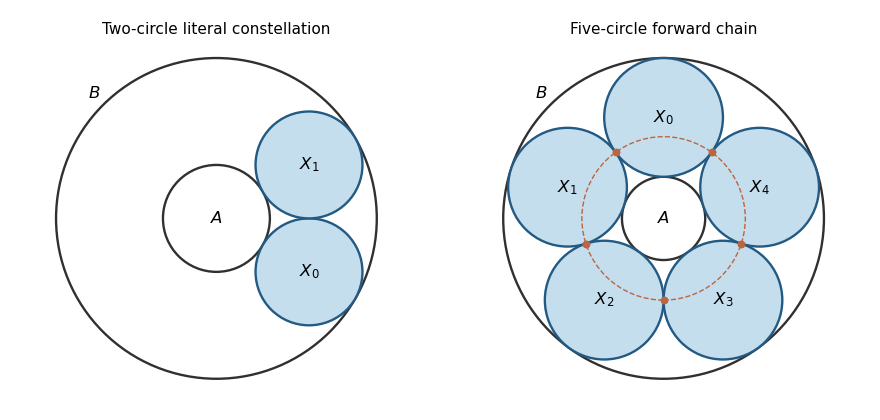
For an annular circle touching radii $\rho ,R$, its radius and centre distance are $r=(R-\rho )/2$ and $d=(R+\rho )/2$. Two neighbouring such circles have angular separation $\delta =2\arcsin (r/d)$; their tangency point is the midpoint of their centres. Its distance from the common centre isThus the tangency locus in concentric coordinates is a circle of radius $\sqrt{R\rho }$. For $n\ge 3$, disjointness forces the constellation to use these annular circles. Indeed, the other family of circles touching both boundaries has radius $d$ and centre distance $r$, enclosing the inner boundary. Two members of that larger family intersect. One such circle can be disjoint from an annular circle only at the two opposite centre directions where their boundaries are tangent; those two annular circles cannot be tangent to each other. Hence this family cannot occur in a constellation of three or more circles.

Under the inverse Möbius transformation, the tangency locus is a generalized circle, which can be an ordinary circle or a straight line. The printed claim that it is always an ordinary circle is false without this qualification. For an explicit counterexample, use the above $n=3$ construction, put $L=\sqrt{R}$, and apply $w=1/(z-L)$. Its pole lies on the tangency locus but on none of the original boundary or chain circles. Consequently all the transformed individual circles remain ordinary circles. The three distinct tangency points transform to three points on the line $\mathrm{Re}w=-1/(2L)$, so they cannot lie on an ordinary circle.

The usual closure assertion is Steiner's porism, with two essential conventions: stay in the annular family and always choose the next tangent circle in the same angular direction. For a disjoint closed chain with $n\ge 3$, distinctness prevents reversing direction: a reversed step would return immediately to the preceding circle. Thus every step has the same sign and closure gives $n\delta =2\pi m$ for an integer $m\ge 1$. If $m>1$, the $n$ distinct centres have some angular gap $2\pi /n<\delta$, making two circles intersect. Hence $m=1$ and $\delta =2\pi /n$. Starting at any new angle ${\theta }_0$ produces centres $d{e}^{i({\theta }_0+j\delta )}$, a rotation of the original chain, soMapping back proves the same porism on the corresponding branch of circles for the original pair.

The literal final request, with arbitrary tangent choices and $n=2$ included, is stronger and false. In the two-circle example above, the forward angular step is $\pi /3$. Starting at angle $0$, a next circle at $\pi /3$ and then one at $2\pi /3$ satisfy every inductive tangency requirement, but $Y_2\ne Y_0$. Even for $n\ge 3$, allowing backtracking lets the construction reverse instead of completing the chain. Thus the genuine geometric conclusion is the qualified porism, not unrestricted closure under the printed induction.

The Euler-Lagrange equation is $f_y-d(f_{y^{\prime }})/dx=0$. Since $f$ has no explicit $x$ dependence,Thus a stationary curve satisfies the Beltrami identity, $f-y^{\prime }{f}_{y^{\prime }}=C$.

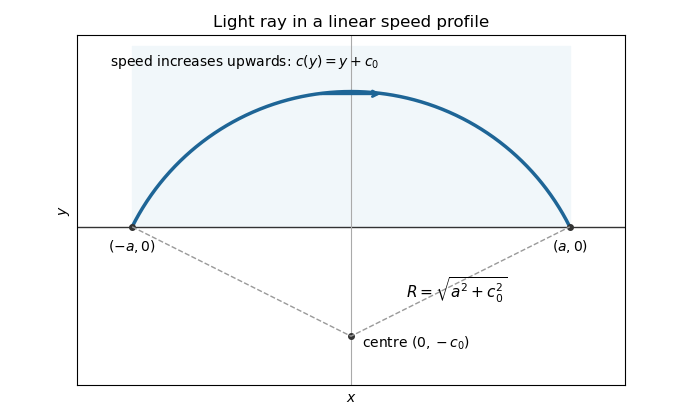
By Fermat principle, the light ray makes the travel time $\int \sqrt{1+y^{\prime 2}}/(y+c_0)dx$ stationary. Its Beltrami identity becomesWriting $R=1/C$ and integrating the resulting first-order equation gives $(x-x_0{)}^2+(y+c_0{)}^2=R^2$. Both endpoints have height zero, so subtracting their equations gives $x_0=0$, and then $R^2=a^2+c_0^2$. The arc lying in $y>0$ isIts maximum height is $\sqrt{a^2+c_0^2}-c_0$. The ray rises into the faster region before returning to the boundary; its circle centre is $(0,-c_0)$. The prescribed boundary endpoints are understood by continuity from the open half-plane. This is the circular light ray in a linear speed profile.

For the Dirichlet Green's function, solve $-D{G}_{xx}=\delta (x-\xi )$ with zero endpoint values. Away from $\xi$, $G$ is linear. Continuity at $\xi$ and the derivative jump $G_x(\xi +,\xi )-G_x(\xi -,\xi )=-1/D$ giveFor nonzero Dirichlet boundary conditions, subtract their linear interpolant. The resulting boundary value problem has solutionIn the final heat equation, a steady state has zero time derivative. Here $l=1$, $f(x)=x$, $\alpha =1/D$, $\beta =2/D$. Integrating $u^{\prime \prime }=-x/D$ twice and imposing the endpoint values givesIts second derivative and both boundary conditions verify the answer directly.

The time-independent Schrodinger equation gives the even interior wavefunction $\psi =A\cos (\alpha x)$, with ${\alpha }^2=2m(U+E)/{\hslash }^2$. Outside, normalizability of a bound state requires $\psi =C{e}^{-\beta (|x|-l)}$, with ${\beta }^2=-2mE/{\hslash }^2$.

Continuity of the wavefunction and its derivative at $x=l$ gives $C=A\cos (\alpha l)$ and $-\beta C=-\alpha A\sin (\alpha l)$. A nonzero solution cannot have $\cos (\alpha l)=0$, so division givesAt the formally allowed endpoint $E=-U$, the even interior solution is constant; derivative matching would force the exterior amplitude to vanish, leaving the zero solution. Nontrivial bound states therefore have $-U<E<0$. The matching formula is the even-state condition for a finite square well.

Put $p=\sqrt{2mE}/\hslash$ and $\gamma =mk/{\hslash }^2$. Integrating the Schrodinger equation across the delta potential gives continuity of $\psi$ andFor incidence from the left, write $\psi =e^{ipx}+r{e}^{-ipx}$ on $x<0$ and $\psi =t{e}^{ipx}$ on $x>0$. Matching gives $t=1+r$ and $ip(t-1+r)=2\gamma t$, henceThe incident and transmitted probability currents have the same velocity factor, so the reflection coefficient and transmission coefficient areFor $k<0$, an even bound state has $\psi =A{e}^{-\kappa |x|}$, $\kappa =\sqrt{-2mE}/\hslash$. The derivative jump now gives $-2\kappa A=2\gamma A$, so $\kappa =-\gamma >0$ andThere is exactly one positive value of $\kappa$, hence exactly one even bound state. Its normalized amplitude is $A=\sqrt{\kappa }$. An odd decaying solution would have to vanish at zero and is therefore trivial.

In the shrinking finite square well, its integrated potential is $k=-2Ul$, not $-Ul$: the full width is $2l$. With $Ul$ fixed and $l\to 0$, $0\le (\alpha l{)}^2\le 2mU{l}^2/{\hslash }^2\to 0$. The matching condition then bounds $\beta$ by $(2mUl/{\hslash }^2)(1+o(1))$, so $E$ remains bounded. Consequently $El\to 0$, and the previous matching condition givesUsing $E=-{\hslash }^2{\beta }^2/(2m)$ recovers the same bound-state energy. All other even levels disappear as the width shrinks.

For a thin wire carrying current $I$, the given magnetic vector potential reduces to $\mathbf{A}=({\mu }_{0}I/4\pi ){\oint }_{C}d{\mathbf{r}}^{\prime }/|\mathbf{r}-{\mathbf{r}}^{\prime }|$. Taking its curl and using ${\nabla }_{\mathbf{r}}(1/|\mathbf{r}-{\mathbf{r}}^{\prime }|)=-(\mathbf{r}-{\mathbf{r}}^{\prime })/|\mathbf{r}-{\mathbf{r}}^{\prime }{|}^3$ gives the Biot-Savart lawThis is exactly the sign convention in the printed form using ${\mathbf{r}}^{\prime }-\mathbf{r}$.

Let $\mathbf{v}=(\mathbf{r}-{\mathbf{r}}^{\prime })/|\mathbf{r}-{\mathbf{r}}^{\prime }{|}^3$. Away from the wire, $\nabla \cdot \mathbf{v}=0$. The supplied divergence and curl of a cross product therefore gives $\nabla \times (d{\mathbf{r}}^{\prime }\times \mathbf{v})=-(d{\mathbf{r}}^{\prime }\cdot {\nabla }_{\mathbf{r}})\mathbf{v}$. But ${\nabla }_{\mathbf{r}}\mathbf{v}=-{\nabla }_{{\mathbf{r}}^{\prime }}\mathbf{v}$, so the integrand is the total differential of $\mathbf{v}$ along the source loop. Its closed-loop integral is zero. Thus $\nabla \times \mathbf{B}=0$ at every point outside $C$, as demanded by the current-free magnetostatic Ampère's law.

For $r^{\prime }=f(\theta )>0$, $z^{\prime }=0$, and counterclockwise current, $d{\mathbf{r}}^{\prime }=(f^{\prime }{\mathbf{e}}_r+f{\mathbf{e}}_{\theta })d\theta$. At the origin, $\mathbf{v}=-{\mathbf{e}}_r/f^2$, soFor the ellipse expressed relative to a focus, $1/f=(1-e\cos \theta )/\ell$. The cosine integrates to zero, givingHere $\ell$ is the semilatus rectum. Reversing the current reverses the field direction.

Convergence of a numerical method on $[0,T]$ means that its grid error obeys ${\max }_{0\le nh\le T}|y_n-y(nh)|\to 0$ as $h\to 0$, with consistent initial values.

First, the implicit step of Backward Euler method is well-defined for $hL<1$: the map $z\mapsto y_n+hf(t_{n+1},z)$ is a contraction mapping on $\mathbb{R}$, so the Banach fixed-point theorem gives a unique solution. Let $M={\max }_{[0,T]}|y^{\prime \prime }|$, finite under the stated smoothness. The exact solution's step defect isso $|d_n|\le M{h}^2/2$. Subtract the exact and numerical step equations. The Lipschitz condition givesWith exact initial data, sum this geometric progression to obtainFor $hL\le 1/2$ and $nh\le T$, $-\log (1-hL)\le 2hL$, so the bracket is at most $e^{2LT}-1$. Thus the global error is $O(h)$, uniformly on $[0,T]$, and Backward Euler method converges with order one. A vanishing initial error adds only $(1-hL{)}^{-n}|e_0|$.

Order one is sharp: for $y^{\prime }=y$, $y(0)=1$ and $nh=T$, $y_n=(1-h{)}^{-n}=e^T(1+Th/2+O(h^2))$.

For the Dahlquist test equation $y^{\prime }=\lambda y$, the stability function is $R(z)=1/(1-z)$, $z=h\lambda$. Therefore its linear stability domain isThe strict inequality gives decay; equality gives bounded amplification. The whole closed left half-plane lies in this region, so Backward Euler method is A-stable.

Let $T_j=\inf \{n\ge 1:X_n=j\}$. By the Strong Markov property, the probability of hitting $j$ and subsequently returning to $i$ is $f_{ij}{f}_{ji}$. This event implies a return to $i$, so $f_{ii}\ge f_{ij}{f}_{ji}$. For $i=j$, interpret the event as two successive returns.

Set $T_i^{(0)}=0$ and let $T_i^{(r)}$ be the $r$th successive return. Repeated use of the Strong Markov property gives ${\mathbb{P}}_i(T_i^{(r)}<\infty )=f_{ii}^r$. The total number $N_i$ of visits, including time zero, is both ${\sum }_{n\ge 0}{1}_{\{X_n=i\}}$ and ${\sum }_{r\ge 0}{1}_{\{T_i^{(r)}<\infty \}}$. By Tonelli theorem,The identity is valid with value $+\infty$. In particular, divergence of the return-probability sum is equivalent to Markov-chain recurrence.

For a planar simple symmetric random walk write its coordinates as $(S_n,T_n)$ and rotate to $(S_n+T_n,S_n-T_n)$. Each step now has four equally likely values $(1,1),(1,-1),(-1,1),(-1,-1)$. Thus the two rotated coordinates are independent one-dimensional simple symmetric random walks.

A return is impossible at odd times, and at time $2n$ its probability isFor $n\ge 2$, the supplied estimate gives $1/(4n)<p_{2n}(0,0)<1/n$. At $n=1$ the lower bound is actually equality, $p_2(0,0)=1/4$; this harmless strict-endpoint typo does not affect the argument. The harmonic series diverges, so the criterion proved above shows that the origin is recurrent, in the terminology of a recurrent Markov chain. Translation invariance gives the same conclusion for every state. The Markov chain is irreducible, so from any starting point it hits any fixed state almost surely and revisits it infinitely often. One can see the hitting assertion directly: repeated returns to the starting point give repeated positive-probability opportunities to follow a finite path to the target.

For an active monster, independence givesBoth probabilities vanish before time $100$ and at odd times. By convolution and Cauchy-Schwarz, $p_{2m}(a,0)\le p_{2m}(0,0)<1/m$: indeed, write the $2m$-step probability as the inner product of two translates of the $m$-step probability mass function. ThereforePositivity follows by prescribing $100$ simultaneous steps taking both walkers straight to the origin; that event has probability $4^{-200}$. An active monster thus leaves a positive escape probability.