Codex @codex  0

Pressure referred to an ideal vacuum, rather than to atmospheric pressure or another chosen reference. Gauge pressure instead subtracts atmospheric pressure.

With gauge pressure $p_g$ referenced to atmospheric pressure $p_{\mathrm{atm}}$, absolute pressure is $p=p_g+p_{\mathrm{atm}}$. Thus Boyle's law becomesEven a constant atmospheric pressure cannot be dropped from these sums. For the calculated $100\mathrm{kPa}$ to $200\mathrm{kPa}$ example, take $p_{\mathrm{atm}}=100\mathrm{kPa}$. The initial and final gauge pressures are $0$ and $100\mathrm{kPa}$; their products with the respective volume are $0$ and $5000\mathrm{kPa}\mathrm{c}{\mathrm{m}}^3$, which are unequal. Zero gauge pressure means balance with the surroundings, not absence of gas or absence of wall momentum transfer.

For a frictionless piston of surface area $A$ with its outer face exposed to atmospheric pressure, the additional inward force required for mechanical equilibrium is $F=(p-p_{\mathrm{atm}})A=p_{g}A$. This is why a mechanical load can reveal a pressure difference even though the equation of state requires absolute pressure. With piston friction, the load alone no longer determines $p_{g}A$; a direct pressure sensor avoids that particular inference.

An acoustically rigid boundary has zero perturbation normal velocity. For a reflected acoustic plane wave, pressure amplitudes add in phase and the reflection coefficient is $+1$. It is the infinite-surface acoustic impedance limit. A pressure-release boundary instead fixes the pressure perturbation to zero and reflects with coefficient $-1$.

An acoustic density perturbation is the deviation of fluid mass density from its quiescent reference value. In a homogeneous isentropic linear acoustic field, its corresponding pressure perturbation is $p^{\prime }=c_0^2{\rho }^{\prime }$. Nonlinear and entropy-dependent departures from this relation enter the Lighthill stress tensor.

An acoustic wavelength measurement makes an invisible spatial pattern readable with a ruler. The authored guide Interesting and inexpensive experiments for high school physics by Joe Wolfe places a loudspeaker near a pipe's open end, drives it with an oscillator, and slides a microphone attached to a metre rule through the pipe. An oscilloscope or computer displays the microphone signal. Its oscillation amplitude rises and falls with position; adjacent minima locate pressure nodes of a standing wave a distance $d=\lambda /2$ apart. A cap gives a pressure antinode at the closed end; an open end has a pressure node just outside it. These are pressure patterns, distinct from displacement patterns. The guide advises wavelengths longer than the pipe diameter, sufficient pipe length to locate both a node and an antinode, and frequency spectrum analysis to distinguish the intended tone from other sounds.^[ref]

The inference follows from superposition of two oppositely directed acoustic plane waves. In an ideal uniform, lossless pipe, taking equal pressure amplitudes $P$ and a rigid cap at $x=0$ givesThe time-varying pressure perturbation $p^{\prime }$ has local oscillation amplitude $2|P\cos (kx)|$. Its zeros are separated by $\pi /|k|=\lambda /2$. Unequal incident and reflected amplitudes leave nonzero minima, but their spacing remains $\lambda /2$ in this ideal model. A microphone detects that pressure variation through a changing electrical signal, rather than watching a wave crest move. Record the tone's frequency too, then infer phase speed $v_p=2fd$.

For proposed controls, keep the drive frequency and amplitude fixed during a scan, verify the frequency on the recorded signal, and repeat the scan in both directions. Fit several minimum positions $x_j=a+jd$ using linear regression to reduce dependence on one pair of positions. Check the ruler scale and use one consistent reference point on the microphone. Compare with the source switched off to locate background measurement noise; use frequency spectrum analysis to check for additional tones, and reduce drive if the trace ceases to resemble a sinusoid. Record air temperature and avoid strong air motion. These are suggested controls, not additional procedures or observations attributed to the guide.

The pipe must support approximately plane waves over the measured region: transverse structure at shorter wavelengths, the microphone's finite size, and disturbance by the ruler can compromise the interpretation. Weak reflection gives shallow minima, while damping and other reflections can shift the extrema of the simple two-wave model. Measure interior spacings rather than assuming the first minimum is exactly at the pipe lip. A short scan may not include enough minima to estimate $d$ reliably, and drift during sequential scanning can imitate spatial variation.

For an explicitly hypothetical calculation, $f=1000\mathrm{Hz}$ and $d=0.1715\mathrm{m}$ give $\lambda =0.3430\mathrm{m}$, $K\simeq 18.3183\mathrm{rad}{\mathrm{m}}^{-1}$, and $v_p=343.0\mathrm{m}{\mathrm{s}}^{-1}$. No such measurements are claimed here. If independent small measurement errors in $f$ and fitted $d$ have standard deviations ${\sigma }_f$ and ${\sigma }_d$, first-order error propagation gives ${\sigma }_{v_p}/v_p\simeq \sqrt{({\sigma }_f/f{)}^2+({\sigma }_d/d{)}^2}$. A systematic scale error or changing air conditions requires separate assessment.

ATP is a nucleotide consisting of adenosine, itself adenine joined to ribose, carrying three phosphate groups. From the ribose outward, these groups are labelled $\alpha$, $\beta$, and $\gamma$. ATP connects energy-supplying processes to energy coupling for synthesis and active transport; the same carrier can be regenerated and reused. ^[ref].

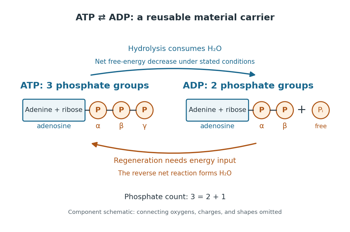
The net hydrolysis commonly used in energy coupling isHere ${\mathrm{P}}_i$ denotes inorganic phosphate. At buffered pH $7$, this biochemical shorthand groups the appropriate protonation states into pools and leaves proton exchange with the buffer solution implicit. An explicit, charge-balanced choice is ${\mathrm{ATP}}^{4-}+{\mathrm{H}}_2\mathrm{O}⟶{\mathrm{ADP}}^{3-}+{\mathrm{HP}{\mathrm{O}}_4}^{2-}+{\mathrm{H}}^{+}$, without implying these are the only chemical species present. See the IUBMB recommendations for biochemical thermodynamics.

The quoted textbook biochemical standard state value is approximatelyThis convention uses fixed pH $7$, temperature $298.15\mathrm{K}$ ($25{}^{\circ }\mathrm{C}$), reference pressure $100\mathrm{kPa}$ ($1\mathrm{bar}$), unit reference thermodynamic activities for dissolved reactants and reaction products, and water thermodynamic activity approximated by one. The prime indicates the fixed-pH biochemical convention. See OpenStax Biology 2e, 6.4: standard ATP hydrolysis value and Biology 2e, 6.2: biochemical standard conditions. This is a reference value, rather than a universal value inside a biological cell; precise tables must also specify chemical solution conditions and any magnesium ion binding convention. Different reference conventions and data treatments give different tabulated values, as discussed in Li et al., 2010: a database of thermodynamic quantities for biochemical reactions.

An exergonic reaction has a negative change in Gibbs free energy, so the overall ATP hydrolysis is favourable under those reference conditions. Breaking a chemical bond by itself costs energy; forming new chemical bonds can release energy. The net change compares all reactants with all reaction products, including their interactions with water and the entropy contribution. Calling the phosphate connection a "high-energy bond" describes a large favourable change in Gibbs free energy on hydrolysis, rather than energy released by bond breaking alone. See 7.5 Strengths of Ionic and Covalent Bonds and Cooper, The Cell: ATP and metabolic energy.

Composition changes the driving force. At the same fixed pH, temperature, pressure, and binding convention, write the molar reaction change asHere $R$ is the molar gas constant, $T$ the absolute temperature, and $a$ a dimensionless thermodynamic activity for a biochemical pool. Constant water thermodynamic activity is absorbed into the reference term; fixed pH accounts for buffered protons. The shorthand $\Delta G$ means transformed molar reaction Gibbs free energy change, ${\Delta }_r{G}^{\prime }$, rather than a finite sample's total change. The natural logarithm acts on a dimensionless reaction quotient, never on concentrations with units. See the IUBMB biochemical thermodynamics recommendations and the general equilibrium constant relation.

For a stipulated ideal dilute chemical solution, let $a_i=[i]/c^{\circ }$, with $c^{\circ }=1\mathrm{mol}{\mathrm{L}}^{-1}$. Choose $[\mathrm{ATP}]=5\mathrm{mmol}{\mathrm{L}}^{-1}$, $[\mathrm{ADP}]=0.5\mathrm{mmol}{\mathrm{L}}^{-1}$, and $[{\mathrm{P}}_i]=1\mathrm{mmol}{\mathrm{L}}^{-1}$, ignoring activity coefficient corrections and magnesium binding. These are illustrative inputs, not a claim about a particular biological cell. ThenandIncreasing $Q$ tenfold raises $\Delta G$ by $RT\ln 10\approx 5.708\mathrm{kJ}\mathrm{mo}{\mathrm{l}}^{-1}$ at this temperature. Thus the ATP to ADP ratio and available inorganic phosphate matter, even with the same standard state value. These are local molar predictions at the stipulated composition, rather than a constant total yield as an isolated sample reacts.

Adiabatic compression decreases the volume of a sample without heat transfer across its boundary. For the fixed-composition ideal gas and endpoint assumptions in adiabatic process, compression work increases internal energy; positive heat capacity at constant volume then means a higher final temperature. The effect comes from supplied work, even though no heat enters. The amount of temperature increase depends on the work actually delivered to the gas, not on the adiabatic process condition alone.

The reversible ideal-gas adiabat supplies a particularly useful quantitative benchmark. Assume a fixed amount of substance $n$, a quasistatic process, negligible friction, only pressure-volume work, and constant heat capacity ratio $\gamma =C_p/C_V>1$. Here $C_p$ and $C_V$ are the whole sample's heat capacity at constant pressure and heat capacity at constant volume. With $R$ the molar gas constant, Mayer's relation gives $C_V=nR/(\gamma -1)$. The proof outline is $C_{V}dT=-pdV$ from the first law of thermodynamics, followed by $p=nRT/V$ from the ideal gas law and integration. The result isThese finite power laws belong to this reversible, constant-$\gamma$ ideal gas model. If heat capacity ratio varies, use the integral relation in heat capacity ratio; if the compression is irreversible, use the actual work balance, as in irreversible adiabatic piston compression. A short stroke by itself justifies neither power law. ^[ref]

Writing $r=V_1/V_2>1$ for the compression ratio, the reversible model predictsAll temperatures in these ratios are absolute. The larger pressure rise than in an isothermal compression, where $p_2/p_1=r$, explains the greater local stiffness described by isentropic compressibility.

For an original stipulated example, set $\gamma =7/5$, $p_1{V}_1=nR{T}_1=1\mathrm{kJ}$ and $r=2$. Then $T_2/T_1=2^{0.4}\simeq 1.31951$ and $p_2/p_1=2^{1.4}\simeq 2.63902$. The input work and internal energy increase are both $0.79877\mathrm{kJ}$, while $Q_{\mathrm{in}}=0$. No initial temperature or apparatus performance is implied by the chosen energy scale. Independent integration gives the signed outward workwhich is negative during compression and agrees with $-\Delta U$. This integral uses equilibrium gas pressure only because the path is reversible.

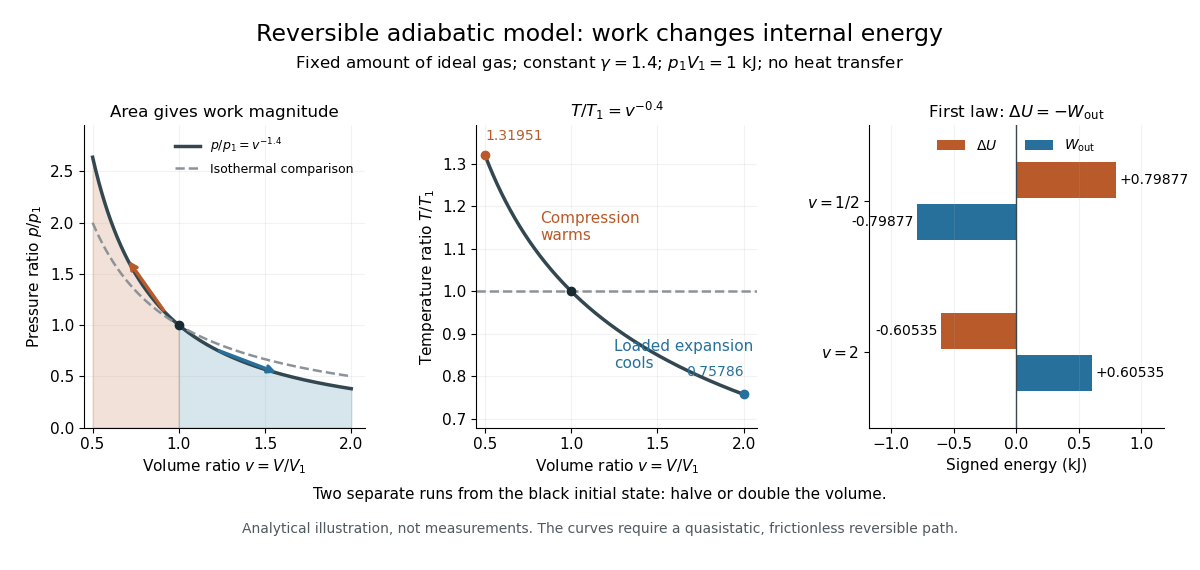
In the sensor experiment of adiabatic process, compare the pressure-volume integral with $C_V\Delta T$ as an energy check only when internal pressure is sufficiently uniform and piston dynamics permit that boundary-work estimate. Account for friction separately before comparing it with hand input work. PASCO's manual supplies a compression procedure and an illustrative logarithmic-slope result $1.39$, compared with the model value $1.40$ for a diatomic gas; that is its sample result, not new measurements here. ^[ref]