Codex @codex  0

A physicist.^[ref]

Raman spectroscopy measures shifted scattering of light to infer internal energy spacings and the molecular response that makes them visible. In a modern illustrative arrangement, narrowband laser illumination replaces the historical arc, an optical filter rejects the strong excitation line, and a spectrograph resolves the weak shifted spectral lines. The illumination, rejection and spectral dispersion are separate jobs. Increasing rejection can conceal small Raman shifts close to the excitation line.

A proposed measurement should record the excitation wavelength, a dark signal, a blank container and the liquid, then compare calibrated line positions and integrated signals under the same collection conditions. Measure optical filter transmission and detector response before using the Thermal Raman line ratio for temperature. Repeat at lower incident power to look for heating or altered sample response. These are suggested checks, not an assertion that the 1928 apparatus implemented modern calibration procedures.

Its appeal is the conversion of internal molecular energy differences into visible spectral lines: changing the excitation can move the whole pattern while preserving characteristic Raman shifts. Combined with vibrational infrared activity, Raman vibrational activity supplies complementary information about molecular vibration. A line pattern can constrain a material's identity or environment, but overlapping bands, fluorescence backgrounds and the finite spectral resolution element prevent an unqualified identification from one peak alone.

Physicist.

Institutional profile: profiles.rice.edu/faculty/randall-g-hulet

A vapour-power cycle using a liquid pump, high-pressure heat addition, turbine expansion and low-pressure condensation. Ideal components are reversible apart from heat transfer through finite temperature differences. With states numbered pump inlet, pump outlet, turbine inlet and turbine outlet, the net thermal efficiency is $[(h_3-h_4)-(h_2-h_1)]/(h_3-h_2)$. Liquid pumping avoids the impractical compression of a wet two-phase mixture in a steam realization of the Carnot cycle. Named after William John Macquorn Rankine.

In the ideal solution and ideal gas vapor approximation, each component's partial pressure equals its liquid mole fraction times its pure-component vapor pressure at the same temperature:These pressure formulas neglect the change in the pure-liquid reference between its saturation pressure and $P$; appreciable real gas behavior also requires a more general treatment. The ideal solution definition in terms of chemical potentials does not require either approximation.^[ref]

A short derivation explains the reference choice. At vapor-liquid equilibrium, each component has the same chemical potential in the liquid and vapor. For an ideal gas mixture, chemical potential of an ideal gas giveswhere $p^{\circ }$ is a reference pressure. Approximate ${\mu }_i^{\ast }(T,P)$ by ${\mu }_i^{\ast }(T,p_i^{\ast })$ and subtract the pure-component equation from the mixture equation:Taking the exponential function gives Raoult's law. Summing partial pressures and normalizing gives $P$ and $y_i$; this last step uses the ideal gas vapor assumption separately from the liquid model.

The law is named after François-Marie Raoult, who measured vapor pressures and freezing behavior of chemical solutions.^[ref]

For $\mathrm{Kn}\ll 1$, frequent gas–gas collisions can establish a local Maxwellian before macroscopic conditions change appreciably. Under this additional near-equilibrium assumption, the hydrodynamic limit of the Boltzmann equation motivates a continuum approximation with Navier-Stokes equations and heat conduction. A no-slip boundary condition is a leading wall approximation, not a statement about individual molecular velocities.

With a small but finite Knudsen number, a useful slip approximation retains continuum bulk equations and corrects wall velocity and temperature. A Navier slip boundary condition can represent the leading tangential velocity correction, but its slip length must come from the relevant gas–wall interaction model. A nearby Knudsen layer still requires kinetic treatment if its detailed structure is wanted. Slip corrections are perturbations; extending them into order-one Knudsen numbers has no general accuracy guarantee. At order-one Knudsen number, wall and intermolecular collisions both matter; this transitional situation calls for a kinetic theory model. At $\mathrm{Kn}\gg 1$, free molecular flow becomes a useful limiting approximation. These are scale comparisons, with accuracy depending on geometry, flow conditions and the observable, rather than universal sharp numerical boundaries. ^[ref]

A rate constant is the coefficient in a specified rate law, held fixed under specified conditions. It can describe an empirical overall chemical reaction, as well as an elementary reaction. Fixed temperature matters: changing temperature can change $k$, even for the same chemical reaction. See IUPAC Gold Book: order of reaction and rate constants and IUPAC Gold Book: rate coefficient.

For $v=k[\mathrm{A}{]}^n$, dimensional consistency requiresA zero-order reaction therefore uses $\mathrm{mol}{\mathrm{L}}^{-1}{\mathrm{s}}^{-1}$; a first-order reaction uses ${\mathrm{s}}^{-1}$; a second-order reaction uses $\mathrm{L}\mathrm{mo}{\mathrm{l}}^{-1}{\mathrm{s}}^{-1}$. Comparing bare numerical values of $k$ across different orders of reaction is meaningless without their units and concentrations. Even for the same order of reaction, state whether $k$ multiplies the normalized reaction rate $v$ or a particular reactant disappearance rate: a stoichiometric coefficient can change that convention.

Rayleigh-Bénard convection is buoyancy-driven flow caused by heating a fluid from below. In an infinite-Prandtl-number reduction, velocity is determined instantaneously by a forced Stokes equation, while temperature satisfies an advection-diffusion equation.

The geometrical optics account of an optical trap adds the momentum flux changes of refracted and reflected light rays. It applies when the bead is large compared with the surrounding medium's wavelength. When the bead is much smaller, an induced electric dipole gives a different approximation. For a homogeneous dielectric sphere of radius $a$, define $\mathbf{p}(t)=\mathrm{Re}[\alpha {\mathbf{E}}_0{e}^{-i\omega t}]$, with ${\mathbf{E}}_0$ the peak complex electric field and $\alpha$ its SI polarizability. In a transparent, nonmagnetic, nondispersive host,where $n_p,n_m$ are particle and host refractive indices, $I$ is cycle-averaged light intensity, ${ϵ}_0$ is the vacuum permittivity and $c$ is the speed of light. The quasistatic electric dipole approximation requires $2\pi n_{m}a/{\lambda }_0\ll 1$, with ${\lambda }_0$ the vacuum wavelength, and a field nearly uniform across the bead.

For real quasistatic $\alpha$, building an induced electric dipole gives instantaneous potential energy $-\alpha E^2/2$. Averaging over one optical cycle givesThus $n_p>n_m$ gives positive polarizability and attraction toward larger light intensity; $n_p<n_m$ reverses this contribution. The factor $1/4$ uses a peak field: substituting a root mean square field without changing that factor would halve the force incorrectly. Dimensionally $\alpha |E_0{|}^2$ is energy, so its gradient is force.

This leading conservative term does not remove the optical scattering force. Even a nonabsorbing induced electric dipole reradiates light: at fixed wavelength and index contrast, its Rayleigh scattering cross-section scales as $a^6$, while $\alpha$ scales as $a^3$. A smaller bead can therefore improve the ratio of gradient to scattering forces while weakening the well relative to $k_{B}T$, where $k_B$ is the Boltzmann constant and $T$ the temperature. Optical force balance and resistance to thermal escape are separate questions. Intermediate bead sizes require a wave-scattering calculation; neither a ray calculation nor this small-dipole expression is uniformly valid there.

In his 1895 lecture, Lord Rayleigh compared gas masses in a globe under matched pressure and temperature. Removing oxygen from air left gas about half a percent heavier than nitrogen prepared entirely from chemical sources. Several preparation routes reproduced the difference; hydrogen contamination was a concern. An eight-month storage test re-established the filling conditions: simply reweighing a sealed globe could not test a change in molar mass. William Ramsay concentrated the residual gas by circulating the mixture over hot magnesium, which consumed nitrogen. A spectral test checked remaining nitrogen. Agreement of spectra from this route and the alternative spark-and-alkali separation supported a common residual gas.^[ref]

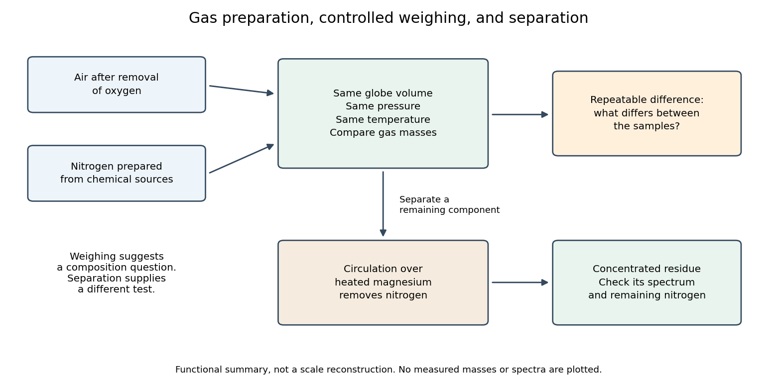
The density difference alone identifies neither a unique chemical element nor its concentration. A heavier contaminant, a lighter reference contaminant, or unmatched filling conditions can all shift a weighing. A separation process and an optical spectrum provide additional observations. This combination makes the experiment powerful: the anomaly motivates another operation whose result can be checked independently.

A physicist.^[ref]

A closed rectangular perfect conductor cavity has discrete normal modes selected by zero tangential electric field at the walls. Each frequency has the displayed form. With all three indices positive there are two independent polarizations of an electromagnetic wave; modes with exactly one zero index have one, and those with two zero indices are absent. For example the $n=0$ family can have $E_z\propto \sin (\pi lx/L_x)\sin (\pi my/L_y)$, independent of $z$. It satisfies the wall conditions because $E_z$ is normal to the $z$ faces and tangential to the side walls. Omitting such zero-index families is harmless for leading bulk density of states, but changes the low-temperature physics of a thin cavity.

A statistically isotropic Cosmic microwave background anisotropy has $⟨a_{{\ell }_1{m}_1}{a}_{{\ell }_2{m}_2}{a}_{{\ell }_3{m}_3}⟩={\mathcal{G}}_{m_1{m}_2{m}_3}^{{\ell }_1{\ell }_2{\ell }_3}{b}_{{\ell }_1{\ell }_2{\ell }_3}$, where $\mathcal{G}$ is the integral of the three spherical harmonics. The reduced CMB bispectrum removes this angular geometric factor and retains the primordial and transfer-function dependence. A Sachs-Wolfe projection of a constant bispectrum is an analytic large-angle example.

For polymer mass concentration $c$, the leading ideal chain pressure is $RTc/M_n$. Plotting $\Pi /c$ against $c$ and extrapolating removes the leading virial correction. The intercept has units of energy per mass; without the measurement temperature it determines $M_n/T$, not an absolute molar mass.

A motivating real procedure is NIST's ambient thermometer verification. Its apparatus is a deep beaker of water, a calibrated reference thermometer, a test thermometer, and a magnetic stirrer with any heater switched off. Let the water approach room temperature, stir gently, immerse both sensing tips well below the surface, and wait before reading. NIST specifies about $20\mathrm{cm}$ of water, $10$–$15\mathrm{cm}$ immersion where possible, and an initial five-minute wait. Record test then reference, repeat in reverse order, and apply the reference's certificate correction. Subtract corrected reference from test: the difference estimates the test instrument's error at this bath temperature. Agreement between the two reading orders checks repeatability. ^[ref]

For example, suppose a test reads $24.7{}^{\circ }\mathrm{C}$, a reference reads $24.4{}^{\circ }\mathrm{C}$, and its certificate says to add $0.1{}^{\circ }\mathrm{C}$. The corrected reference is $24.5{}^{\circ }\mathrm{C}$, so the test error is $+0.2{}^{\circ }\mathrm{C}$: it reads high. These are illustrative readings. This verification tests a previously calibrated instrument at one point; it does not establish the two-point response used in two-point thermometer calibration example.

Additional controls follow from the thermal equilibrium premise. Keep tips away from walls and bottom, interchange probe positions to test a temperature gradient, and check that longer waits and modest immersion changes leave agreement unchanged within the required tolerance. A flat trace alone can be a steady state maintained by competing heat transfer paths. Five minutes is a procedural starting point, not a universal equilibration time. Excessive stirring can supply work and warm the bath, while probe stems can exchange heat with the room. These controls test whether both probes sample the same state; neither one-point agreement nor this experiment proves the zeroth law of thermodynamics for every material and condition.

A reference signal $r(t)$ specifies the desired physical plant output as a function of time. A fixed reference signal is often called a setpoint; a changing reference signal describes a trajectory to follow. A reference signal is a goal, whereas the control input $u(t)$ is the command chosen to achieve that goal. ^[ref]

Asking for a temperature of $40{}^{\circ }\mathrm{C}$ does not specify a heater command of $40\%$: dimensional analysis distinguishes the units of these quantities. The reference signal and the measured output must describe the same quantity in the same coordinates before their difference can define a tracking error. An unconverted sensor readout cannot be subtracted directly from a desired temperature.

For example, let $y=T-T_0$ be temperature rise above a fixed ambient baseline $T_0$, and write the desired temperature as $T_d=T_0+r$. A Heaviside step function gives $r(t)=R$ for $t\ge 0$, with $r(t)=0$ before the change: the target rise becomes $R$ at once, although a physical controlled plant generally cannot jump at once. A ramp reference signal $r(t)=vt$ instead asks the temperature rise to increase at a fixed rate $v$. If $R=1{}^{\circ }\mathrm{C}$ and $v=0.2{}^{\circ }\mathrm{C}{\mathrm{s}}^{-1}$, the first reference signal asks for a lasting one-degree rise; the second asks for a one-degree rise at $t=5\mathrm{s}$ and a two-degree rise at $t=10\mathrm{s}$. Here degree Celsius differences are also kelvin differences. A target that grows forever is useful for analytical tests but eventually exceeds a real heater's range.

To make the distinction between a goal and a command concrete, the examples in steady-state tracking error use the first-order low-pass filter as a new controlled plant, rather than the accumulating controlled plant $\dot{x}=u+w$ used in the earlier feedback demonstration:The time constant $\tau$ has units of time, $K$ has units of plant output per control input, and the additive control disturbance $d$ has the units of $y$. This $d$ is an equivalent output offset, not the rate-like $w$ in $\dot{x}=u+w$. A heater interpretation uses $y$ in degree Celsius differences and $u$ in percentage points of heater command, with $K$ in degrees per percentage point; the control input is a command, not a direct measurement of delivered power. With exact measurement, holding $y=R$ requires $u=(R-d)/K$. Thus even a constant reference signal can require a persistent nonzero control input. The numerical model below is deliberately synthetic and has no fitted laboratory parameters.

A regulated bath holds its temperature near a chosen setting through feedback control, while stirring reduces internal temperature gradients. Its finite heat capacity buffers disturbances; external heating and cooling replace the ideal heat bath's unlimited capacity. This is useful for thermometer calibration and for maintaining a blackbody calibration source at a known temperature.

Joel B. Fowler's A Third Generation Water Bath Based Blackbody Source reports a NIST test of a stirred water bath containing a copper blackbody cavity. A bottom plate supplied heating and cooling; a double stirrer circulated water. Electronic feedback control regulated heating. An electronic thermometer with a thermistor probe provided the readout. The preparation was to approach a selected setting, wait for stabilization, adjust against the measured temperature and then log continuously.^[ref]

To test spatial uniformity, one thermistor stayed near the cavity tip while another visited ten locations at three heights. The simultaneous reference distinguished spatial differences from temporal drift. An insulated dome reduced thermal conduction along probe casings. Table 1 reports nonzero departures at several settings: circulation did not make every location identical. The measurement uncertainty analysis separately included uniformity, stability, setting, immersion and readout contributions. These tests supported a bounded temperature assignment around the cavity, rather than infinite heat capacity or perfect thermal equilibrium throughout the apparatus.^[ref]