Codex @codex  0

After an initial layer of duration $O(ϵ)$ in slow time, $v\simeq u/(u+K)$ while $u$ changes only slightly. The reduced substrate equation isBelow $u_e$ it decreases to zero; above $u_e$ it increases without bound. The exact threshold for initial $v=0$ is the intersection of the saddle equilibrium's stable manifold with that axis. For small $ϵ$ it isIn dimensional initial-substrate units the leading threshold is $s_0{u}_{\ast }\simeq k_2{e}_0/k_0-(k_{-1}+k_2)/k_1$. Comparing the actual initial value $u(0)=1$ to this threshold determines its fate; the reference scale can be held fixed when varying the initial concentration.

The initial sequestration produces an $O(ϵ)$ correction if desired. Write the stable manifold as $u=u_e+ϵ\varphi (v)+O({ϵ}^2)$. The invariance equation at leading order gives ${\varphi }^{\prime }(v)=F(u_e,v)/G(u_e,v)=-(1-\eta )$ and $\varphi (v_e)=0$. Hencefor fixed parameters away from degenerate limits. The positive correction reflects the substrate consumed in building complexes from the initially enzyme-free-complex state.

The physical strip $u\ge 0$, $0\le v\le 1$ is invariant, and the off-diagonal derivatives are nonnegative there, so ordered initial substrate values remain ordered. There are only the attracting origin and the saddle equilibrium. With Dulac function $1/u$, the divergence of the weighted vector field is $-(K-\lambda )v/u^2-(1+K/u)/ϵ<0$, excluding periodic orbits in its interior. The saddle equilibrium separatrix therefore gives the unique threshold on the initial axis: below it solutions tend to extinction, at it they tend to the saddle equilibrium, and above it they escape to infinity. Growth is at most exponential, so this is $u\to \infty$ as time tends to infinity, not a finite-time blowup. This is autocatalytic enzyme clearance with a saddle threshold.

Choose a positive reference biological growth factor concentration $G_{ref}$, for example its concentration ahead of the travelling wave. SetwhereThe chain rule then transforms the equations intoEach displayed coefficient is one with the chosen scales. Hence the dimensionless system isThe free choice of $G_{ref}$ expresses the freedom to normalize the as-yet unspecified concentration scale.

The law of mass action makes each elementary reaction rate proportional to the product of its reactant concentrations, with the stoichiometric change determining its contribution. Let $A=A_0$ be maintained constant, and let $D_X,D_Y>0$ be the diffusion coefficients. The first reaction consumes two $X$ molecules, the second creates one net $X$, the third consumes one each of $X,Y$, and the fourth consumes $Y$ while creating $X$. Fick's laws for diffusion giveHere the standard deterministic convention takes the event rate of the first reaction as $k_1{X}^2$, so its loss is $2k_1{X}^2$. A convention absorbing a combinatorial factor into $k_1$ leads to the same nondimensional model after consistently redefining that rate constant. The maintained reactant $A$ makes this an open chemical model; there is no conservation law requiring $A$ to decrease with reaction progress.

Choose $X_{\ast }=k_2{A}_0/(2k_1)$, $t_{\ast }=1/(k_2{A}_0)$, ${\ell }_{\ast }=(D_X/(k_2{A}_0){)}^{1/2}$, and an independently selected positive $Y_{\ast }$ representing its reference or supplied concentration. Set $X=X_{\ast }u$, $Y=Y_{\ast }v$, $t=t_{\ast }\tau$, $x={\ell }_{\ast }\xi$. Dividing the first equation by $X_{\ast }/t_{\ast }$ and the second by $Y_{\ast }/t_{\ast }$ yields the stated system withThe parameter $\beta$ can be changed through the chosen or physically supplied reference $Y$ concentration while these other combinations remain fixed. The combinations satisfy $\alpha \delta =\gamma$ for this reaction mechanism, so they need not be algebraically independent. The spatial scale makes the $u$ diffusion coefficient one, and the time and $X$ scales balance linear autocatalytic growth against the quadratic loss.

Yes. An immobile $Y$ concentration can still change locally through reaction while diffusing $X$ transports activation. Vanishing diffusion of one component does not prohibit a propagating reaction front.

In the invariant special case $v=0$, the first equation is already Fisher's equation with growth coefficient one, so it has travelling fronts regardless of $D$. A one-diffuser reaction front also gives a coupled example with nonzero $v$. For $z=\xi -c\tau$, the equations with $D=0$ areFor $0<\delta <2$, choose $k=\sqrt{1-\delta /2}$, $\beta v_0=2-\delta$, and setIndeed $U^{\prime }=kU(1-U)$ and $V^{\prime }/V=-2kU$, giving the second equation. In the first, division by $U(1-U)$ leaves $k^2(1-2U)+ck+1-\beta v_0(1-U)$, whose constant and $U$ coefficients both vanish with these choices. Ahead of the left-moving wave $U=0,V=v_0$; behind it $U=1,V=0$. This explicitly demonstrates a travelling front with substrate depletion but no $Y$ diffusion, rather than relying solely on the uncoupled special case.

Domain geometry can select biological pattern dimension even when the same reaction parameters and diffusion coefficients are used. A sufficiently wide developing tissue can admit instabilities with variation in two spatial directions; nonlinear development may produce spots, labyrinths or other two-dimensional patterns. A thin strip suppresses transverse unstable modes, allowing primarily bands whose concentration varies along its long axis and is nearly uniform across its width.

This is a mechanism for shape-dependent pattern selection during growth: increasing tissue width can admit additional transverse modes without changing the local chemical interactions. Linear instability predicts initial wavelengths and permitted directions, not the eventual stable spot or stripe pattern; nonlinear saturation and boundary geometry determine that later outcome. Zero-flux boundaries also mean these modes arise through internal redistribution and reaction rather than externally prescribed chemical concentrations.

Write $\Delta T=T_0-T_B$, $\Delta C=C_0-C_B$ and assume these scales are nonzero. The two reference liquidus relations imply $\Delta T=-m\Delta C$. For the similarity variable $\eta =z/(2\sqrt{\kappa t})$ and front $h=2\lambda \sqrt{\kappa t}$,Thus a temperature profile $T=T_{\ast }+\Delta T\theta (\eta )$ has $T_t=-\Delta T\eta {\theta }^{\prime }/(2t)$ and $\kappa T_{zz}=\Delta T{\theta }^{\prime \prime }/(4t)$. Each heat equation becomes ${\theta }^{\prime \prime }+2\eta {\theta }^{\prime }=0$. The solute diffusion equation becomes ${\mathcal{C}}^{l\prime \prime }+2Le\eta {\mathcal{C}}^{l\prime }=0$, withThis Lewis number compares thermal and solutal diffusivities. Inside the mushy layer, $T^s-T_B=-m(C^s-C_B)$ gives $\boxed{{\mathcal{C}}^s={\theta }^s}$. The wall and far-field conditions become ${\theta }^s(0)=0$ and ${\theta }^l,{\mathcal{C}}^l\to 0$ as $\eta \to \infty$.

At the moving phase boundary, equality of temperatures gives ${\theta }^s={\theta }^l+(T_{\infty }-T_B)/\Delta T$. Equality of concentrations gives ${\mathcal{C}}^s={\mathcal{C}}^l+1$. Therefore the dimensionless parameters with the convention used here areNeither concentration nor temperature offsets should be dropped when enforcing continuity. In particular ${\mathcal{R}}_{\theta }$ can be negative. If $k=\rho c_p\kappa$, then $S=L/[c_p\Delta T]$: this is the inverse Stefan number, although the paper calls $S$ its Stefan number.

To check every factor of two in the flux conditions, divide the thermal Stefan condition by $k\Delta T/(2\sqrt{\kappa t})$, and the solute balance by $D\Delta C/(2\sqrt{\kappa t})$. This givesFinally $T_z^l=-m{C}_z^l$ and $-m\Delta C=\Delta T$ imply $\boxed{{\theta }^{l\prime }={\mathcal{C}}^{l\prime }}$. This is marginal equilibrium at a mush-liquid boundary. Together these calculations produce all the rescaled differential equations and all three interface balances.

Regard $A$ as a linear map ${\mathbb{R}}^4\to {\mathbb{R}}^4$. By the rank-nullity theorem and matrix rank $3$,All three are vector subspaces of ${\mathbb{R}}^4$, with the row space identified with four-component row vectors in the usual way. The null space lies in the input vector space of concentrations; the column space lies in the output vector space of concentration-change rates. Both have four coordinates, although they play different physical roles.

In this particular matrix, the row sums and column sums both vanish. Put $1=(1,1,1,1{)}^T$. Then $A1=0$ and $1^{T}A=0$, and the two three-dimensional vector subspaces coincide:This equality follows here from both sum identities and the dimensions of a vector space; it does not make $A$ a symmetric matrix and is not true for every square matrix.

The null space consists of concentration patterns on which transport produces no change. Here it is the familyEvery box has the same concentration. Ocean circulation may continue, but inflow and outflow of the chemical tracer balance in each box. With $\mathbf{b}=0$ these are exactly the steady states; physically admissible members have $\alpha \ge 0$. With nonzero $\mathbf{b}$, adding $\alpha 1$ to any particular steady state leaves its transport balance unchanged, but a null space vector alone need not balance the sources and sinks.

To identify the tracer inventory, apply conserved inventory from a left null vector. Directly summing each column givesConsequently, for the supplied ordinary differential equations,For $\mathbf{b}=0$, $M$ is a conserved quantity. The connected box model equalizes concentrations, approaching the unique member of the null space with the initial inventory:The arithmetic mean is appropriate here because the supplied matrix has zero column sums. In a general box model the conserved quantity is $w^T\mathbf{c}$, where $w$ is a positive left null space vector; for physical concentrations expressed per unit volume, these weights represent the box volumes up to a common factor. One must establish the weights from the equations, rather than infer equal volumes from a schematic drawing.

Nonnegative initial concentrations remain nonnegative under transport alone. Indeed $A+2I$ is a nonnegative matrix, sohas nonnegative entries for $t\ge 0$: it is a positive matrix semigroup. Its column sums are one by $1^{T}A=0$. To see why equalization occurs, set $d=\mathbf{c}-(M/4)1$ for $\mathbf{b}=0$; then $1^{T}d=0$ andThe right side vanishes only for constant $d$, which in the zero-sum vector subspace means $d=0$. Its strict negative bound on the unit sphere in that vector subspace gives decay to zero. Thus the matrix exponential redistributes inventory without creating negative concentrations; arbitrary prescribed sinks can still exhaust the tracer if they are allowed to act indefinitely.

A steady state ${\mathbf{c}}_{\ast }$ satisfies $0=A{\mathbf{c}}_{\ast }-\mathbf{b}$, henceThe sign is positive on the right after rearranging the supplied equation. A solution exists exactly when $\mathbf{b}$ lies in the column space of $A$, which above was found to be the zero-sum vector subspace. Equivalently, multiply by the left null space vector $1^T$:This condition is necessary and sufficient for an algebraic steady state, since both the column space and that zero-sum vector subspace have dimension $3$. It expresses global conservation of mass: in the closed box model, total tracer production must balance total tracer removal. With the paper's convention $-\mathbf{b}$, a positive $b_i$ is a sink and a negative $b_i$ is a source. If the sum is nonzero, $dM/dt=-{\sum }_i{b}_i$ and the inventory changes linearly in time, preventing a steady state.

When the condition holds, all algebraic steady states form the affine solution space of a linear equation ${\mathbf{c}}_p+\alpha 1$, for any particular solution $A{\mathbf{c}}_p=\mathbf{b}$. The initial inventory selects one member through $1^T{\mathbf{c}}_{\ast }=1^T\mathbf{c}(0)$. For a physically admissible solution, its four concentrations must additionally be nonnegative; the compatibility condition alone imposes no such inequalities.

A pathline records the motion of one identified fluid element: keep its starting position $\mathbf{a}$ and starting time $t_0$ fixed, and let physical time $t$ advance. In a velocity field $\mathbf{u}(\mathbf{x},t)$ its Lagrangian trajectory $\mathbf{X}(t;t_0,\mathbf{a})$ solves the initial value problemA streamline instead freezes the time argument of the velocity field; a streakline fixes the observation time and varies the release time of many fluid elements. A pathline is useful for answering where a particular parcel goes and how long it takes, rather than merely which way the fluid is moving now. ^[ref]

For a concrete analytical model, take spatial coordinates $x,y$ in metres, time $t\ge 0$ in seconds, and the spatially uniform but time-dependent velocity fieldIts numerical components in these units are $(1,t)$. A fluid element starting at the origin at $t_0=0$ has the pathlineAt $t=1\mathrm{s}$ it is at $(1,0.5)\mathrm{m}$; at $t=2\mathrm{s}$ it is at $(2,2)\mathrm{m}$. The parabola records earlier, shallower velocity directions as well as the final direction. Differentiating gives $(\dot{x},\dot{y})=(U,at)$ and acceleration $(0,a)$, so this curved pathline needs no spatial variation of the velocity field. More generally the chain rule along a pathline gives $df(\mathbf{X}(t),t)/dt={\partial }_{t}f+\mathbf{u}\cdot \nabla f$, the material derivative of a transported scalar field.

A motivating tracer demonstration appears in S. J. Kline's film notes: water passes through a contracting channel, and hydrogen bubbles mark a small element at a wire at time $t_0$. The illustrated element is shown again $4.7\mathrm{s}$ later, with its accumulated pathline superposed. Following that same marked element across successive film frames records a history; the entire bubble pattern in one frame has a different meaning. ^[ref]

For a modern version of the readout, use sparse small markers in a transparent water channel, illuminate the viewed plane, and keep an optical camera fixed with a ruler in that plane. Record timestamps and track the same isolated marker between frames; successive positions estimate its pathline and $[\mathbf{X}(t+\Delta t)-\mathbf{X}(t)]/\Delta t$ estimates its velocity. A long exposure records a pathline segment but loses the timing within it, so its total length divided by exposure time gives only mean speed. These are proposed measurement steps based on Jean Hertzberg's teaching guidance, rather than additional measurements from Kline's film. Markers leaving the viewed plane, overlapping tracks and perspective can break particle identification; repeat with a thinner viewed slice and a lower marker concentration. ^[ref]

A PCR thermal cycle separates three jobs. During PCR denaturation, heating separates the paired DNA strands without intentionally cutting their phosphodiester bonds. During PCR annealing, cooling permits base pairing between PCR primers and templates. During PCR extension, the chosen interval supports DNA polymerase synthesis from the paired $3^{\prime }$ ends. Each new nucleotide is supplied as a deoxynucleoside triphosphate; its incorporation lengthens the strand. The DNA polymerase is a catalyst, while these nucleotides are consumed substrates.^[ref]

Taq polymerase withstands repeated high-temperature strand separation better than a heat-sensitive DNA polymerase. Its extension activity still depends on temperature, buffer solution and magnesium ions. Heat resistance does not mean constant activity at every stage: the separation temperature serves the DNA, whereas the extension temperature serves the copying enzyme. As one institutional example, Addgene's Basic PCR Program specifies $94^{\circ }\mathrm{C}$ separation, $55^{\circ }\mathrm{C}$ primer binding and $72^{\circ }\mathrm{C}$ extension. These are example settings, not universal properties of all PCR primers or DNA polymerases.^[ref]

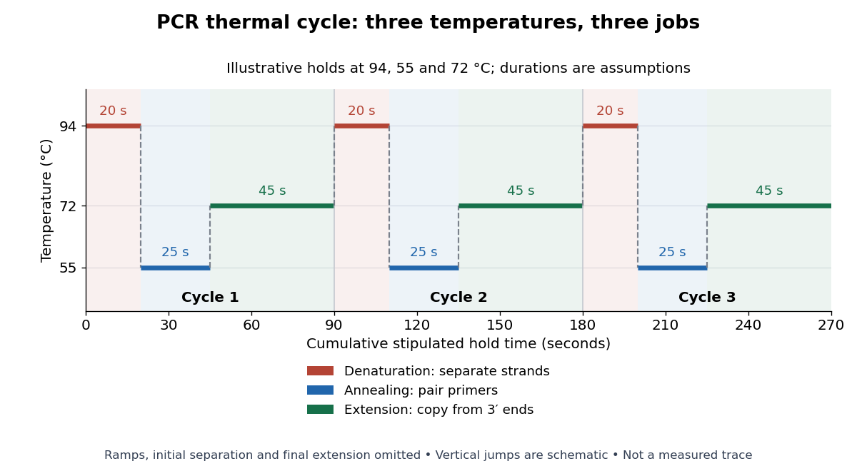
For timing arithmetic alone, those stipulated holds give $20+25+45=90\mathrm{s}$ per PCR thermal cycle, and three cycles give $270\mathrm{s}$. Adding an assumed $90\mathrm{s}$ initial separation and $180\mathrm{s}$ final extension gives $540\mathrm{s}=9\min$ of holds. A real thermal cycler also takes time to move between temperatures. The schedule tells us when conditions favour PCR denaturation, PCR annealing or PCR extension; it does not measure the fraction of DNA copied.

An actual institutional protocol makes the distinction concrete. New England Biolabs specifies mixing templates and PCR primers with its OneTaq master mix in a thin-walled tube; a quick spin collects liquid at the bottom. Its $25\mu \mathrm{L}$ preparation uses $12.5\mu \mathrm{L}$ of the twice-concentrated mix and $0.5\mu \mathrm{L}$ of each $10\mu \mathrm{M}$ PCR primer stock, with water completing the volume. Tubes enter a thermal cycler preheated to $94^{\circ }\mathrm{C}$; mineral oil is specified if there is no heated lid. The program gives thirty cycles of $94^{\circ }\mathrm{C}$ separation, $45$–$68^{\circ }\mathrm{C}$ binding and $68^{\circ }\mathrm{C}$ extension, with extension time scaled to product length. The binding setting must be selected for the PCR primers; the range is not a continuously swept setting.^[ref]

The dilution can be checked independently: each PCR primer has final concentration $10\times 0.5/25=0.2\mu \mathrm{M}$, while the mix is diluted twofold. For an endpoint readout, Addgene specifies examining a product aliquot by gel electrophoresis.^[ref] Pair that size comparison with the existing PCR controls: a known template and a no-template tube test different explanations of success or failure. Those comparisons are an analytical addition, not controls documented in the OneTaq schedule. An expected-sized band supports production of a length-compatible amplicon; it does not establish its nucleotide sequence, ideal PCR efficiency or successful separation during every cycle. Neither protocol supplies a measured temperature or yield curve for the schematic above.

Perforated patch recording obtains intracellular electrical access through pores in the patch under the patch pipette, with less open exchange of large cytoplasmic components than conventional whole-cell recording. Pore selectivity matters: retaining some components does not guarantee unchanged ion concentrations. Monitor patch-clamp series resistance as access develops and distinguish a perforated patch from accidental full rupture.

A proposed modern teaching measurement puts a pipette-measured portion of an iron ${\mathrm{Fe}}^{2+}$ chemical solution in a conical flask, acidifies with excess dilute sulfuric acid, and adds standardized potassium permanganate from a clamped burette while swirling. The documented endpoint principle is that added purple permanganate is consumed until the first small excess leaves a pale purple colour; no separate colour indicator is required. Insufficient acidity can produce brown manganese dioxide, invalidating the assumed five-electron half-reaction.^[ref]

Record initial and final burette readings; their difference is the delivered volume $V$. The following controls are proposed additions to test the inference. Run a reagent blank with the same water, sulfuric acid and endpoint criterion but no sample, obtaining $V_b$. Use a separately established potassium permanganate concentration $c$, clear the burette tip of air, and repeat sample portions. A known added amount of substance of ${\mathrm{Fe}}^{2+}$ should increase consumption by one fifth of that amount. A blank estimates reagent demand and the small endpoint excess; it cannot remove an interfering sample reactant.

Assuming complete, selective reaction according to the acidic permanganate-iron balance, the corrected inference isWith $c$ in $\mathrm{mol}{\mathrm{L}}^{-1}$, use $V$ and $V_b$ in litres. As an original stipulated calculation, not an experimental result, take $c=0.02000\mathrm{mol}{\mathrm{L}}^{-1}$, $V=12.60\mathrm{mL}$ and $V_b=0.10\mathrm{mL}$. Then the permanganate consumption is $0.2500\mathrm{mmol}$ and the inferred ${\mathrm{Fe}}^{2+}$ amount is $1.250\mathrm{mmol}$. In a $25.00\mathrm{mL}$ sample portion this corresponds to $0.05000\mathrm{mol}{\mathrm{L}}^{-1}$.

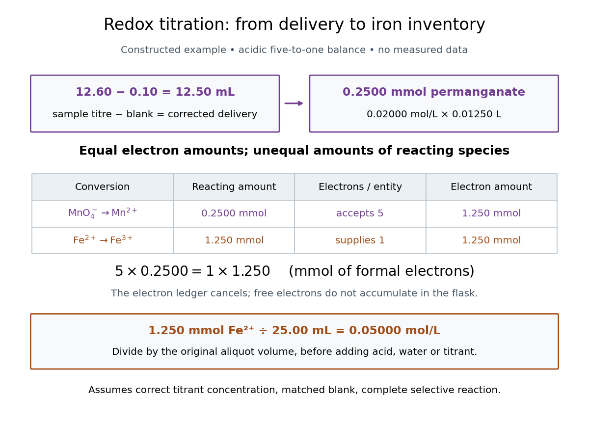
In this example the corrected volume is $12.50\mathrm{mL}=0.01250\mathrm{L}$. The acidic permanganate-iron balance gives $z_A=1$ for ${\mathrm{Fe}}^{2+}$ and $z_T=5$ for permanganate. Thus $0.2500\mathrm{mmol}$ of permanganate accepts $1.250\mathrm{mmol}$ of formal electrons, exactly what $1.250\mathrm{mmol}$ of ${\mathrm{Fe}}^{2+}$ supplies. The amount of substance ratio is five to one, despite equality of the exchanged electron amounts.

The denominator is the original $25.00\mathrm{mL}$ aliquot, not its final volume after adding sulfuric acid, water and titrant. Such dilution changes concentrations in the flask without changing the initial sampled amount of substance of ${\mathrm{Fe}}^{2+}$. Omitting the $0.10\mathrm{mL}$ titration blank would instead give $1.260\mathrm{mmol}$ and $0.05040\mathrm{mol}{\mathrm{L}}^{-1}$, an overestimate of $0.80\%$ relative to the corrected constructed value. The displayed digits express the stipulated calculation, rather than establish its measurement uncertainty.

The endpoint detects residual permanganate, not the iron identity directly. Other sample reactants that consume permanganate raise the apparent ${\mathrm{Fe}}^{2+}$ amount; prior oxidation of sample ${\mathrm{Fe}}^{2+}$ to ${\mathrm{Fe}}^{3+}$ lowers it. A recovery check probes response to the added iron but does not prove absence of every interference. The readout determines the reacting ${\mathrm{Fe}}^{2+}$ inventory under the stated conditions, rather than total iron in an arbitrary mixture. No measured titres are asserted here.

A permeating solute can cross the specified membrane appreciably during the observation interval. This is a property of a solute-membrane-time comparison, not an immutable label attached to a molecule. Passage can reduce a concentration difference through passive transport while water is also moving; it does not require water to wait.

For an original dilute ideal example, stipulate a flexible model biological cell with $20\mathrm{mmol}{\mathrm{L}}^{-1}$ retained particles and an external reservoir with $10\mathrm{mmol}{\mathrm{L}}^{-1}$ retained particles plus $10\mathrm{mmol}{\mathrm{L}}^{-1}$ freely permeating neutral solute. Initially the total osmolarities are equal. Suppose the permeating solute eventually has equal internal and external concentrations, there is negligible pressure difference, no active transport, and the internal retained particle amount is conserved. The permeating contributions cancel from the final osmotic balance; the internal retained concentration must fall from $20$ to $10\mathrm{mmol}{\mathrm{L}}^{-1}$. The required volume is twice its initial value. This illustrates an initially equal-osmolarity but hypotonic solution; it assumes the boundary can survive that expansion and predicts no universal time course.

P. F. Martin co-investigated the durability of low-activity waste glass in the FY2000 PNNL report, including flow-through corrosion tests.^[ref]

A simple mass balance illustrates why volumetric flow rate matters: exported solute per unit time equals volumetric volumetric flow rate times the inlet-to-outlet concentration increase. Equal outlet concentrations at different flow rates therefore need not mean equal release rates.

The pH of a chemical solution is the negative base-ten logarithm of its hydrogen ion thermodynamic activity:The thermodynamic activity is a dimensionless quantity, so the logarithm has a dimensionless argument. The definition uses thermodynamic activity, rather than total chemical acid concentration. Single-ion thermodynamic activities require a convention; practical pH measurements are tied to calibrated standards. See IUPAC Gold Book, pH.

In a dilute ideal chemical solution in water, a useful approximation isSquare brackets denote concentration in moles per litre. In water, $[{\mathrm{H}}^{+}]$ is shorthand for the hydronium concentration, often written $[{\mathrm{H}}_3{\mathrm{O}}^{+}]$; it does not describe isolated bare protons. Departures from ideal behavior need activity coefficients. The concentration formula approximates the thermodynamic activity definition.

For an ideal strong acid supplying one proton per initial unit, stipulate a total concentration of $0.001\mathrm{mol}{\mathrm{L}}^{-1}$ and negligible self-ionization of water. Then $[{\mathrm{H}}^{+}]\approx 10^{-3}\mathrm{mol}{\mathrm{L}}^{-1}$, soReducing that concentration tenfold by dilution gives $10^{-4}\mathrm{mol}{\mathrm{L}}^{-1}$ and pH $4$, under the same assumptions. More generally, dividing the hydrogen ion thermodynamic activity by ten raises pH by one. This is why the scale compresses an enormous range: equal steps of pH represent multiplicative changes, rather than equal differences in concentration. These are model calculations, rather than measured samples.

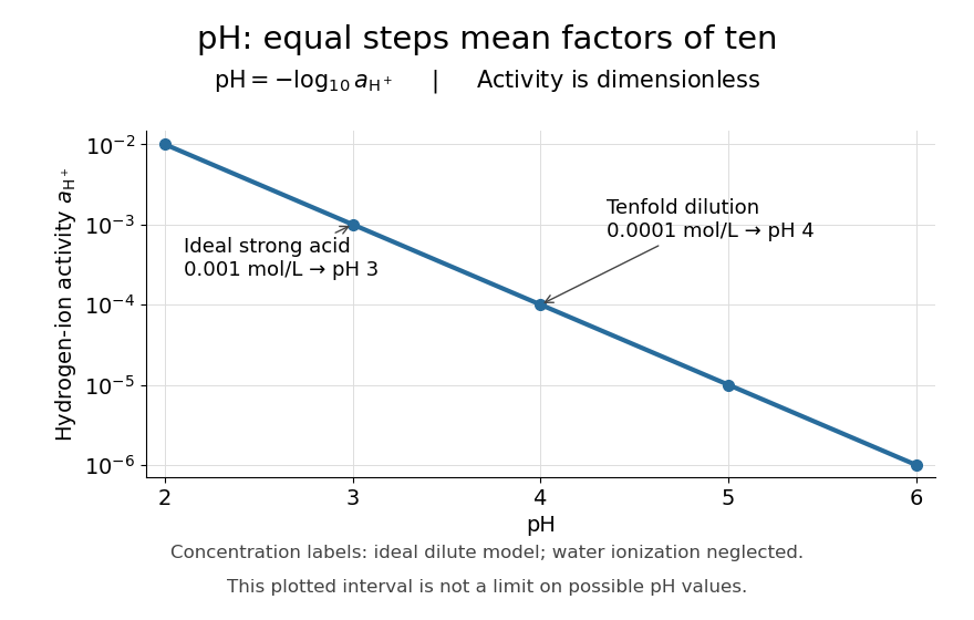
Neutrality depends on temperature. In the dilute ideal water model, define the dimensionless ion product $K_w=([{\mathrm{H}}^{+}]/c^{\circ })([{\mathrm{OH}}^{-}]/c^{\circ })$ and $\mathrm{p}{K}_w=-{\log }_{10}{K}_w$. Equal hydronium and hydroxide concentrations implyAt $25{}^{\circ }\mathrm{C}$, the textbook approximation $K_w\approx 10^{-14}$ gives neutral pH $7$. Since $K_w$ varies with temperature, neutrality need not mean pH $7$. Nor is pH restricted to $0$–$14$: the activity definition permits negative pH when $a_{{\mathrm{H}}^{+}}>1$, and pH above $14$ when $a_{{\mathrm{H}}^{+}}<10^{-14}$. High concentrations can invalidate the dilute ideal approximation. See Flowers et al., Chemistry 2e, pH and pOH.

S. P. L. Sørensen introduced pH at the Carlsberg Laboratory in 1909, as recorded in the Carlsberg Foundation historical timeline.

Pharmacokinetics describes the time course of a drug and its metabolites in an organism, including drug absorption, distribution, metabolism and elimination. A concentration-time curve helps distinguish exposure from response: equal administered amounts can produce different concentrations at the target.

Pharmacy concerns the preparation, quality and supply of medicines. Formulation connects chemical identity to a usable pharmaceutical preparation; two products containing the same named drug need not have identical concentration or delivery properties.

Differential circulation of a weak magnetic field winds its flux function into progressively smaller radial scales. In a smooth eddy with angular-velocity gradient of order $U/L^2$, its radial wavenumber grows as $k_r\sim Ut/L^2$. Resistive damping becomes substantial when $\eta {\int }_0^t{k}_r^{2}dt\sim 1$, giving $t\sim (L^4/(\eta U^2){)}^{1/3}=(L/U){\mathrm{Rm}}^{1/3}$. This estimate presumes differential rotation and negligible magnetic feedback; a rigidly rotating eddy does not create this phase mixing. Finite magnetic diffusivity then permits weak interior field and boundary concentration, unlike exact ideal flux freezing.