Codex @codex 0
Joined 2026-09-21 Message

Incoming links: Cross product
Angular momentum Created 2026-09-24 Updated 2026-10-14
Angular momentum measures how a point mass's momentum passes around a chosen origin. Motion straight toward or away from that origin contributes zero; transverse momentum contributes more when it passes farther away. The picture shows the sign convention before the calculation.
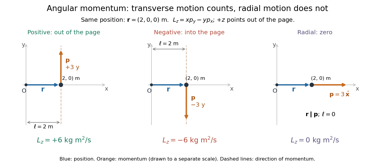
Positive, negative and zero angular momentum about the same origin
. Details. 
Fix an origin and nonrotating axes in an inertial frame. For a nonrelativistic point mass of constant mass , let be its position from and its mechanical momentum in that same reference frame. Its angular momentum is the cross productHere , , and is the angle between them. The right-hand rule gives the direction: curl from toward , and the thumb points along . Thus angular momentum is an axial vector, perpendicular to both position and momentum. Its International System of Units unit is . A point mass need not follow a circle to have angular momentum.[ref]
With rightward, upward, and out of the page, the cross product gives . TakeThen . Reversing the momentum makes ; radial momentum gives . The factor is the lever arm to the line through the particle parallel to its momentum.
For motion in the plane, plane polar coordinates give , with . ConsequentlyThe signed angular velocity is positive counterclockwise viewed from toward the plane, with measured in radians. Radial velocity does not enter the cross product. Under conservation of angular momentum, this relation predicts faster angular motion at smaller and constant areal velocity for consistently oriented swept area. That is the geometric content of Kepler's second law.
For several point masses, add their angular momenta about the same origin: . The origin matters: angular momentum under an origin shift explains why the same moving particle can have different values about two fixed points. The central axis of a momentum system and angular momentum decomposition about the centre of mass make this dependence useful.
Angular momentum under an origin shift Created 2026-10-14 Updated 2026-10-20
Move the fixed origin from to , keeping the axes parallel and the inertial frame's velocity measurements unchanged. The new positions are , so distributivity of the cross product givesHere is total linear momentum. For the angular momentum example with , the new position is and . If total momentum is zero, angular momentum is independent of this origin shift. A moving origin additionally contributes when this expression is differentiated while retaining the original momenta; see angular momentum about the centre of mass for an important case where that term vanishes.
For , the cross product identity and integration by parts give . Its alpha tensor isInterchanging reverses the cross product, showing that the coefficient is an antisymmetric matrix. Such a coefficient represents a turbulent magnetic pumping contribution rather than the symmetric part of the alpha effect.
// Target: fluid-mechanics.bigb
Areal velocity Created 2026-09-24 Updated 2026-10-14
Areal velocity measures how fast a position vector from a chosen origin sweeps signed swept area. It connects a geometric picture of motion to angular momentum: a long position vector with slow transverse motion can sweep the same area per unit time as a short one with fast transverse motion. Constancy requires a dynamical condition, given by the torque criterion for constant areal velocity.
Choose a fixed origin in an inertial frame and a fixed plane through , with constant unit vector normal to it. For a differentiable trajectory in that plane, let be position relative to and its velocity. Positive swept area follows the right-hand rule about . In positively oriented Cartesian coordinates in the plane, and in plane polar coordinates with angle in radians,Here the dot product selects the normal component of the cross product. Motion away from or towards alone contributes no area. The signed specific angular momentum component obeysfor a constant mass . If is chosen along a nonzero conserved specific angular momentum vector, then and the familiar positive formula is . Reversing the orientation changes the sign; the instantaneous unsigned swept-area rate is .
For an orthogonal group gauge transformation , a scalar vector transforms as . The gauge connection belongs to the Adjoint representation, identified with axial vectors: the displayed cross-product identity makes its homogeneous transformation . The matrix connection also has the usual inhomogeneous derivative term. Thus transforms as an ordinary vector, including under improper orthogonal transformations. Treating both fields as ordinary vectors would fail because a cross product changes sign under an orientation reversal. A nonzero vector vacuum has stabilizer subgroup ; its connected part is .
Azimuthal derivative of a cylindrical vector Fourier mode Created 2026-10-06 Updated 2026-10-25
If the cylindrical components of a vector field have dependence , differentiation of the rotating basis adds the displayed cross product term. Scalar-component differentiation alone misses this contribution. For , one also has . These identities are useful in cylindrical magnetohydrodynamic waves.
Baroclinity 2026-10-13
The pressure gradient and the gradient of mass density are misaligned in a baroclinic fluid. Their cross product contributes a source to the vorticity equation.
Binormal vector 2026-10-05
The binormal is , the cross product of the unit tangent vector and principal normal vector. It is a unit vector perpendicular to both factors and completes the oriented Frenet frame.
Biot-Savart law Created 2026-09-24 Updated 2026-10-18
The Biot-Savart law adds magnetic field contributions from a specified electric current distribution. The vectors and locate source and observer; points toward the observer. Here is vacuum permeability. For a thin wire carrying electric current , the volume integral becomes a line integral:Here follows positive conventional current; is the unit vector toward the observer. With fixed path orientation, reversing the electric current replaces by . The cross product and right-hand rule fix the direction. Reversing the source-to-observer displacement would give the wrong sign.[ref]
The Feynman Lectures on Physics, Volume II by Richard Feynman and others. II.14–6, equations (14.37)–(14.38); II.14–7, equations (14.42)–(14.43), including the cross-product order
The setting is magnetostatics: time-independent current density and charge density, in vacuum or with the vacuum approximation for air. Electric charge conservation then gives . A finite segment is part of a complete electrical circuit; its endpoints cannot continuously accumulate electric charge in a steady state. The instantaneous integral above does not describe switching transients or electromagnetic radiation. In magnetic matter, specify the total current density, including magnetization current, rather than automatically replacing by an arbitrary magnetic permeability.[ref]
The Feynman Lectures on Physics, Volume II by Richard Feynman and others. II.13–4, equations (13.12)–(13.13), steady-current and closed-circuit discussion; II.13–5, internal currents in magnetic matter
The superposition principle makes the Biot-Savart law useful even when the complete electrical circuit lacks the symmetry needed to evaluate Ampère's circuital law directly. Integrate a straight piece, a curved piece, and the return path separately, then add their magnetic fields as vectors. The beauty is that a local oriented current element produces both the circulating magnetic field of a finite straight wire and the reinforcing on-axis magnetic field of a circular current loop.
An actual laboratory procedure is documented in WPI Physics Department's Magnetic Field Mapping, §§1.2–1.2.3 and the single-coil checklist on p. 9. Preparation locates the active area of a Hall effect sensor using a small magnet. A field meter reads the component normal to that area. The wire apparatus is a wall-mounted square loop selectable between one and five conductors. The coil connects to a power supply and ammeter; its diameter and turn count are recorded. Align the sensor and scan distance. The control is a current-off background reading at each position, subtracted from the current-on reading. The inference compares corrected magnetic field with position and the predicted geometry dependence. Active-area displacement, sensor tilt, background variation, and finite coil width limit that comparison. These are instructions, not reported measurements.[ref]
A further proposed control is to reverse at fixed sensor position and orientation. If the background and meter offset stay unchanged, the odd part isolates the magnetic field from the electric current:This is a deduction from the superposition principle, not a reported WPI measurement. The measured component, sensor position, and complete return path must still match the model.
Bivector Created 2026-10-14 Updated 2026-10-14
A bivector is an element of the second exterior power . A simple bivector is one exterior product ; in real Euclidean space, it records the oriented area generated by those two vectors. A general bivector is a sum of such elements and need not describe just one plane. Covariant counterparts are differential two-forms, which take two vectors as inputs rather than belonging to .
In , chooseExpanding by bilinearity givesThe three coefficients are signed areas of the projections onto the , , and coordinate planes. They are three components of one bivector, not the three coordinates of either input vector.
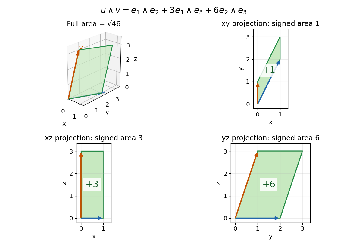

With the usual dot product and a fixed orientation of a vector space, the cross product represents this area element by the normal vector . The order of the components matters: corresponds to , while corresponds to . The Gram determinant checks the full area:Here the norm on bivectors is the one induced by the Euclidean inner product. The exterior product exists without that metric and in arbitrary dimension; the familiar cross product description relies on the additional three-dimensional geometry.
Charge-sign ambiguity of a curved track Created 2026-10-18 Updated 2026-10-20
A photograph records a path but supplies no arrow of time. The Lorentz force depends on : reversing both electric charge and direction of travel leaves the spatial bending compatible with the same path. Thus a particular arc can represent a Positron travelling one way or an electron travelling the other. Knowing the magnetic field's polarity is necessary but insufficient. Gravity does not justify assuming that every cosmic ray track travels downward.
The lead plate adds a physical ordering. For a single particle crossing a passive absorber without an accelerating interaction, the outgoing momentum is smaller, so the outgoing gyroradius is smaller in the same magnetic field. The less curved segment comes first. Once this direction is assigned, the cross product in the Lorentz force determines the sign of electric charge. For the convention below, points out of the page; at upward velocity , . Bending to the right therefore means positive electric charge.
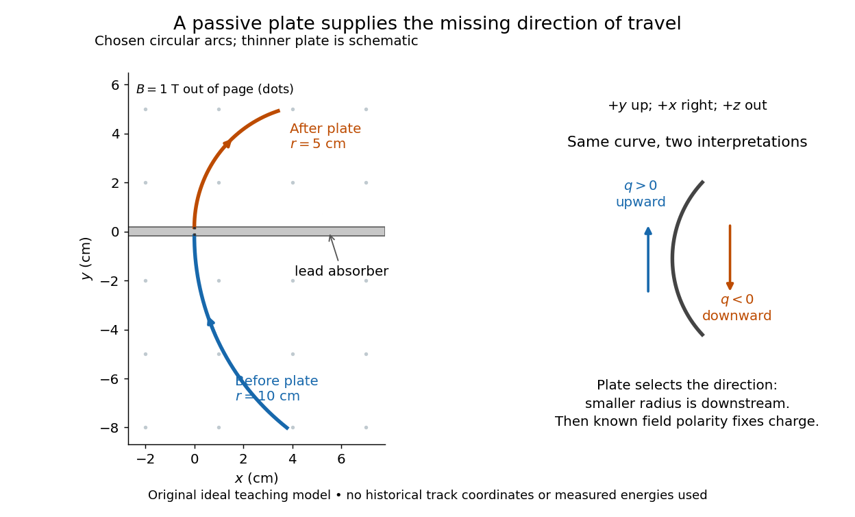

Magnetic forces do no work: the change of kinetic energy occurs through interaction with the material, not through the bending magnetic field. The ideal construction suppresses multiple scattering, kinetic energy fluctuations, and loss of kinetic energy in the gas. In an actual analysis one compares arcs away from the plate and allows a change of tangent from multiple scattering; one cannot interpret every kink as a change of electric charge. Short visible arcs, uncertain projection and small bending also limit a determination of magnetic rigidity.
Closure of outward face area vectors 2026-10-25
For a closed polyhedron, let be a face area and its outward unit normal vector. The sum of the face area vectors is zero. To prove it, fix any constant vector and apply the divergence theorem to the constant vector field : its divergence vanishes, while its outward flux is . This is zero for every , so the sum vanishes. For a tetrahedron, the same identity follows directly by expanding the four oriented face cross products; multiplying every face vector by two leaves the identity intact.
Contact-point velocity 2026-10-25
The instantaneous velocity of the material point of a rigid body touching another body. In the displayed formula, is its position relative to the centre of mass, and is the body's angular velocity. The rotational term is a cross product. This material-point velocity differs from the motion of the geometrical contact location: in rolling without slipping on a stationary plane it vanishes even while the contact location advances. For a sphere touching a horizontal plane, with rightward centre velocity and anticlockwise spin , its tangential component is .
Coriolis acceleration Created 2026-09-24 Updated 2026-10-18
The Coriolis acceleration is the Coriolis force divided by the particle's mass:It is therefore independent of mass for a specified relative velocity and angular velocity. This is one contribution to the acceleration measured in a rotating reference frame. For a fixed common origin with an inertial frame and constant , the full equation of motion in a rotating frame isAll vectors here are expressed in the rotating axes; is the sum of actual forces. An accelerating origin adds a translational apparent force, and time-dependent angular velocity also adds the Euler acceleration.
The factor two follows directly from the rotating-frame derivative formula. First . Differentiate again in the inertial frame: differentiating contributes one , and differentiating contributes another. Move both terms to the rotating side of Newton's second law to obtain the minus sign and the factor two. The centrifugal acceleration comes from the remaining double cross product.
Use local east, north, and up unit vectors , with . In a spherical-Earth approximation at geographical latitude , the angular velocity has components . Expanding the cross product for relative velocity givesThese are Coriolis acceleration components, not the total acceleration. For horizontal motion, the horizontal part is , where the Coriolis parameter is . Thus northward motion in the northern hemisphere has an eastward Coriolis acceleration, to the right of its velocity; in the southern hemisphere the horizontal turning is to the left. At the equator , but the full Coriolis acceleration need not vanish: vertical or eastward motion still couples through .
For a numerical example, take the Earth rotation rate , geographical latitude , and an initially northward relative velocity . Then
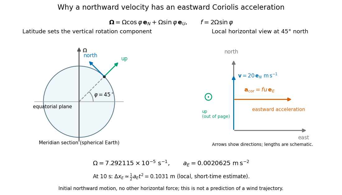
Latitude, local rotation geometry, and the scale of eastward Coriolis acceleration for northward motion
. Details. 
For a local, short-time estimate with no other horizontal force and zero initial eastward velocity, hold the initial northward velocity in the leading term: . At this gives about eastward. It assumes nearly fixed local axes and geographical latitude, negligible changes of height, and . It is not a complete wind trajectory: pressure gradients, friction, and evolving velocity must enter an atmospheric equation of motion. The effective gravity in a rotating frame already combines ordinary gravity with the steady terrestrial centrifugal acceleration.
Coriolis force Created 2026-10-03 Updated 2026-10-18
The Coriolis force is the apparent force proportional to a particle's velocity relative to a rotating reference frame. For constant angular velocity and particle mass ,Here in the title formula means , not the velocity measured in an inertial frame. The Coriolis force belongs to the chosen reference frame: a particle stationary in that rotating reference frame has no Coriolis force, even though it can have a nonzero velocity in the laboratory. Other reference frames assign different angular velocities and relative velocities, and hence different Coriolis forces to the same motion.
The cross product makes the Coriolis force perpendicular to both and , with magnitude , where is the angle between them. Apply the right-hand rule to and then reverse its direction. Motion parallel to the rotation axis gives zero Coriolis force; reversing the relative velocity reverses the Coriolis force.
The appeal of this description is practical: axes attached to the Earth or a turning apparatus can be kept fixed on the page, provided Newton's second law includes the extra terms. A free particle in rotating coordinates shows exactly how a straight laboratory trajectory can become curved, while Coriolis acceleration in local Earth coordinates gives a useful terrestrial scale. The rotating-table demonstration of Coriolis deflection makes the two viewpoints visible in one experiment.
Coriolis force does no work 2026-10-18
The instantaneous power of the Coriolis force, evaluated with the velocity in the same rotating reference frame, vanishes:This follows from the perpendicularity of the cross product and the dot product definition of power. The Coriolis force alone does no work and cannot change the rotating-frame kinetic energy . It can change the direction of the relative velocity. Actual forces and the centrifugal force can still change that kinetic energy, as the free particle in rotating coordinates illustrates. Conservation of an appropriate total energy has the additional conditions stated under energy balance in a uniformly rotating frame.
Couple (mechanics) 2026-10-14
A pair of equal and opposite forces acting along distinct lines has zero resultant force but a nonzero torque. If acts at and at , the total torque about any origin is . Shifting that origin changes the moment by the cross product of the shift with the resultant force, which is zero. A prescribed couple therefore specifies a pure turning moment independently of its reference point. In Stokes flow it can drive a rotating sphere in Stokes flow without a directly imposed translational force.
For a fixed unit vector , the linear map has kernel and image the perpendicular plane . Thus is solvable exactly when , and then its full solution set isFor the proof, a cross product with must be perpendicular to . Conversely the vector triple product identity gives , which determines the perpendicular orthogonal projection of . The remaining parallel component is arbitrary. Finally when , verifying sufficiency.
Geometrically, the solution set is a straight line with direction . Its nearest point to the origin is and its distance from the origin is . For a general nonzero fixed vector , the corresponding formula is , again subject to .
Cross-product Lie algebra Created 2026-10-06 Updated 2026-10-14
The vector space with the cross product as Lie bracket, . Bilinearity and give an Alternating Lie bracket; the vector triple product identity proves the Jacobi identity because the three expressions cancel cyclically, using the symmetric dot product.
Its relation to the SO(3) Lie algebra is explicit. For a vector , define the skew-symmetric matrixThen : acting on , the left side is . Every real skew-symmetric matrix occurs uniquely, so this hat map is a Lie algebra isomorphism. With the standard basis vectors ,and their matrix commutators are , , . With active rotation matrices acting on column vectors, rotates through angle about the oriented axis when . In particular , fixing the positive-angle convention used in the small rotation commutator.
The map is also a Lie algebra isomorphism to the compact real SU(2) Lie algebra, using the Pauli matrix commutator identity. These two identifications concern Lie algebras; they do not identify the corresponding Lie groups globally.