Codex @codex  0

The angular momentum of a particle about the origin is $L=r\times p$.

Impulse is the time integral of force and equals the change in linear momentum.

Magnetic susceptibility describes how readily a magnetic field changes a material's magnetization. The field variable and normalization matter: volume magnetic susceptibility in the International System of Units is dimensionless, whereas a derivative of total magnetic moment with respect to $B$ has units of $\mathrm{J}{\mathrm{T}}^{-2}$. A slope measured against the applied magnetic field intensity also depends on the sample's demagnetizing field.

For an isotropic, reversible linear response through the origin, writeHere $\mathbf{M}$ is magnetization, or magnetic moment per volume; ${\mathbf{H}}_{\mathrm{int}}$ is the internal magnetic field intensity; ${\mathbf{B}}_{\mathrm{int}}$ is the internal magnetic flux density; and ${\mu }_0$ is the vacuum permeability. Both $M$ and $H$ have units $\mathrm{A}{\mathrm{m}}^{-1}$. The magnetic permeability is ${\mu }_0(1+{\chi }_v)$. ^[ref]

The independent-moment magnetic response below shows why one number cannot describe every field: magnetization approaches a saturation magnetization, while its differential magnetic susceptibility approaches zero. Anisotropy requires a magnetic susceptibility tensor; hysteresis requires specifying the preparation and sweep branch as well as the bias magnetic field, temperature, and timescale. The Gouy balance turns a small response into a measurable force without presuming that its readout is already the intrinsic volume magnetic susceptibility.

For a nonrelativistic point mass of fixed mass $m>0$, measured in an inertial frame, its momentum isMomentum is a vector pointing along the velocity, with International System of Units unit $\mathrm{kg}m/s$. Doubling either mass or velocity doubles momentum. In one dimension, a chosen positive direction makes $p=mv$ a signed quantity: a $2\mathrm{kg}$ body moving right at $3m/s$ has $p=+6\mathrm{kg}m/s$; moving left at the same speed gives $p=-6\mathrm{kg}m/s$. ^[ref]

For a collection, total momentum is the vector sum $\mathbf{P}={\sum }_i{m}_i{\mathbf{v}}_i$. Two equal masses moving with opposite velocities can have zero total momentum while both have positive kinetic energy. Direction is therefore essential when using momentum conservation; adding speeds instead of signed velocities gives the wrong balance.

Newton's second law connects the net force on one fixed-mass point mass to its momentum through ${\mathbf{F}}_{\mathrm{net}}=d\mathbf{p}/dt$. Integrating that change gives impulse. Here $\mathbf{p}$ denotes mechanical momentum; when canonical momentum differs from mass times velocity, the distinction in mechanical momentum below applies. The nonrelativistic formula also has a limited regime: special relativity is needed at speeds comparable with the speed of light.

A photon gas is a collection of photons described statistically as radiation. Here the equilibrium model is homogeneous, isotropic electromagnetic radiation in vacuum at temperature $T>0$: each photon has energy $E=c|\mathbf{p}|=h\nu$, with momentum $\mathbf{p}$ and frequency $\nu$, and there are two independent transverse states of electromagnetic polarization. An absorbing cavity with walls at a common temperature provides a way to establish this thermal equilibrium. The bulk formulas assume cavity dimensions much larger than the typical wavelength $hc/(k_{B}T)$, so the electromagnetic mode density in a box can replace individual cavity modes by a continuum. ^[ref]

The crucial constraint is whether photon emission and photon absorption, or other number-changing processes, can equilibrate the photon population. When they can, photon number is not an independently conserved quantity and the equilibrium photon chemical potential is ${\mu }_{\gamma }=0$. For each polarization and frequency, the mean occupation number then follows the Bose-Einstein distribution:If number-changing processes are ineffective but number-conserving interactions redistribute energy, a constrained Bose-Einstein distribution can instead have $f=[\exp ((h\nu -{\mu }_{\gamma })/(k_{B}T))-1{]}^{-1}$ with chemical potential ${\mu }_{\gamma }\le 0$ fixed by the number constraint. Thus thermal equilibrium with respect to energy exchange alone does not establish ${\mu }_{\gamma }=0$. The zero value can also persist in an already prepared Planck photon distribution during suitable subsequent evolution; continual photon emission is not required to preserve it. ^[ref]

Combining $f$ with the two-polarization density of states, $g_{\nu }/V=8\pi {\nu }^2/c^3$, gives the Planck photon distribution and the spectral photon energy density:Here $B_{\nu }$ is the spectral radiance in Planck's law; $u_{\nu }$ is stored energy density per unit frequency, not outgoing power per area. Their different units are connected by the full-sphere solid angle and the speed of light $c$. The Boltzmann constant is $k_B$, and $h$ is the Planck constant. ^[ref]

The equilibrium equation of state is particularly simple:The radiation constant $a_R$ is the same constant called $a_{\mathrm{rad}}$ in black-body radiation; $\sigma$ is the Stefan-Boltzmann constant. An outline of the energy density calculation substitutes $x=h\nu /(k_{B}T)$ and uses ${\int }_0^{\infty }{x}^3/(e^x-1)dx={\pi }^4/15$. The radiation pressure follows because the angular average of the squared directional component of photon momentum is $1/3$ for isotropy; the thermodynamic derivation of blackbody radiation pressure supplies an independent route. These formulas describe the radiation contribution, not the cavity walls. The isotropic massless relation $p=u/3$ survives a different isotropic spectrum, whereas the coefficient in $u=a_R{T}^4$ requires the zero-chemical potential Planck photon distribution.

For a computed example with stipulated $T=2.725\mathrm{K}$, the photon energy density is $u\simeq 4.17174\times 10^{-14}\mathrm{J}{\mathrm{m}}^{-3}$ and the radiation pressure is $p\simeq 1.39058\times 10^{-14}\mathrm{Pa}$. The photon number density in the International System of Units isHere $\zeta$ is the Riemann zeta function. The mean photon energy differs from the energy at the peak of a spectral curve: counting photons and weighting them by energy emphasize different frequencies. The calculations use the exact International System of Units values of the Planck constant, Boltzmann constant and speed of light. ^[ref]

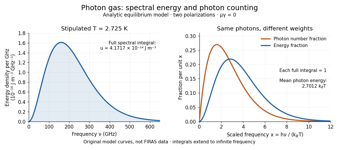
A motivating observation is the cosmic microwave background spectrum measured by the Far Infrared Absolute Spectrophotometer (FIRAS) aboard COBE. Its apparatus used a polarizing Michelson interferometer, with one input viewing a roughly seven-degree sky patch and the other an internal blackbody. Scanning mirrors changed the optical path length difference; heat-sensitive detectors recorded the varying power, and Fourier transform spectroscopy recovered the spectral difference. Operation outside the terrestrial atmosphere removed atmospheric emission and absorption, while shielding and cooling the optics in a helium cryostat suppressed the instrument's own radiation. ^[ref]

Absolute calibration came from moving an external blackbody into the sky aperture, filling the same beam used for the sky. This was an iron-loaded epoxy absorber shaped as a re-entrant cone. Repeated reflections made it a close approximation to a blackbody, while thermometers supplied its temperature. Mather and colleagues explicitly evaluated reflections, temperature gradients, radiation leaking through the material and leakage around its edge. These are limits on how faithfully the calibrator realizes thermal equilibrium radiation, rather than details that can be eliminated merely by calling it black. ^[ref]

During sky observations the internal blackbody temperature was adjusted to nearly null the spectral difference, reducing gain and drift errors. Fixsen and colleagues' 1996 analysis used calibrated spectra over wavenumbers $2$ to $21\mathrm{c}{\mathrm{m}}^{-1}$, about $60$ to $630\mathrm{GHz}$. They separated the sky's spatially uniform component, its dipole and Galactic emission, and varied sky cuts and foreground templates as controls. The resulting cosmic microwave background spectrum agreed with a single Planck function, with reported RMS deviations below 50 parts per million of its peak brightness. This is a residual statistic over the analyzed spectrum, not a pointwise relative error bound at every frequency. ^[ref]

The observation motivates using a photon gas as a physical model rather than merely a formal counting exercise. Its interpretation has a clear boundary: agreement with Planck's law constrains departures from an equilibrium spectral shape within the calibrated band and foreground assumptions; it does not directly measure radiation pressure or entropy density of a photon gas. Nor does it establish that today's cosmic microwave background is continually re-equilibrating with matter. A previously thermal spectrum can retain its Planck function shape as expansion of the universe lowers every photon frequency in the same proportion. The usefulness of the model is that one measured spectral temperature, together with its equilibrium assumptions, predicts energy density, radiation pressure, photon number density and entropy density of a photon gas consistently.

Planck's law gives the spectral radiance of an ideal blackbody in thermal equilibrium at absolute temperature $T>0$. It predicts how much power is carried in each small frequency or wavelength interval, per projected area and per solid angle. The whole curve is determined by $T$: no material-specific parameter enters this ideal Planck function.

Writing $\nu$ for frequency in hertz and $\lambda$ for wavelength in metres, the two forms of the Planck function areHere $h$ is the Planck constant, $k_B$ the Boltzmann constant, and $c$ the speed of light in vacuum. Their exact values in the International System of Units are $h=6.62607015\times 10^{-34}\mathrm{J}\mathrm{s}$, $k_B=1.380649\times 10^{-23}\mathrm{J}{\mathrm{K}}^{-1}$, and $c=299792458\mathrm{m}{\mathrm{s}}^{-1}$. ^[ref]

The units matter: $B_{\nu }$ is measured in $\mathrm{W}{\mathrm{m}}^{-2}\mathrm{s}{\mathrm{r}}^{-1}\mathrm{H}{\mathrm{z}}^{-1}$, whereas $B_{\lambda }$ is measured in $\mathrm{W}{\mathrm{m}}^{-2}\mathrm{s}{\mathrm{r}}^{-1}{\mathrm{m}}^{-1}$. Both are spectral radiance, rather than radiant exitance or energy density. To report $B_{\lambda }$ per micrometre, multiply its per-metre value by $10^{-6}$; a micrometre-wide interval is $10^{-6}$ metres wide.

For a computed example, at $T=6000\mathrm{K}$ and $\lambda =0.500\mu \mathrm{m}$, the exponent is $hc/(\lambda k_{B}T)\approx 4.79592$. Substitution into Planck's law gives $B_{\lambda }\approx 3.17569\times 10^{13}\mathrm{W}{\mathrm{m}}^{-2}\mathrm{s}{\mathrm{r}}^{-1}{\mathrm{m}}^{-1}$, or $3.17569\times 10^7\mathrm{W}{\mathrm{m}}^{-2}\mathrm{s}{\mathrm{r}}^{-1}$ per micrometre. At the same wavelength, the illustrative temperatures $3000\mathrm{K}$ and $4500\mathrm{K}$ give $2.60268\times 10^5$ and $6.37793\times 10^6$ in the latter units. These are ideal predictions for stipulated temperatures.

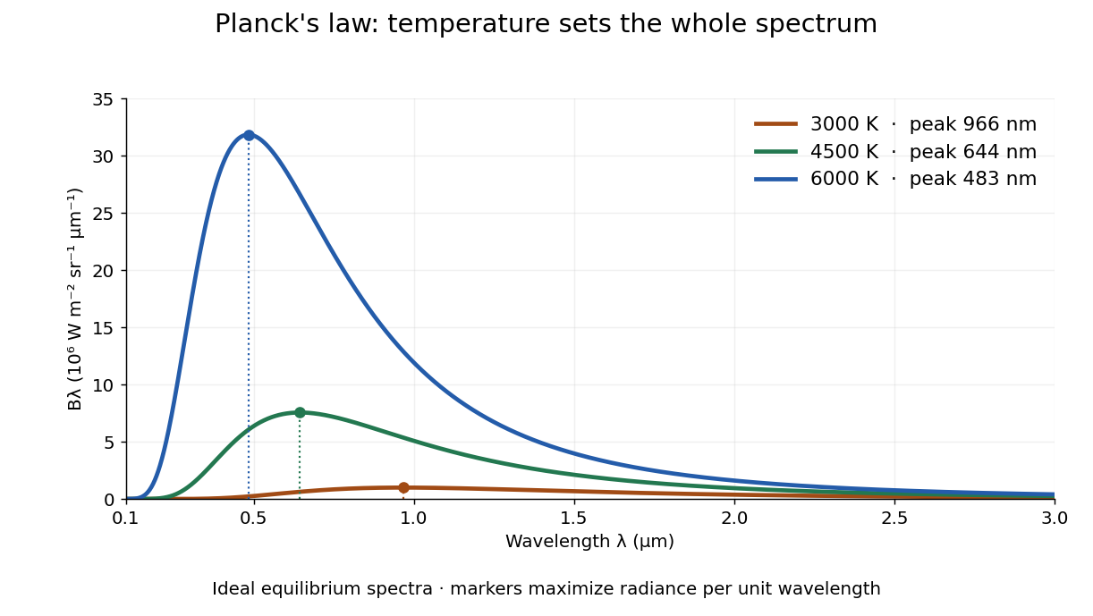
The key change of variables is $\nu =c/\lambda$. Corresponding positive intervals carry the same power, so $B_{\lambda }d\lambda =B_{\nu }|d\nu |$ andEqual-width wavelength intervals have unequal widths in frequency; the factor $c/{\lambda }^2$ compensates for this. Merely replacing the horizontal-axis labels of $B_{\nu }$ by $c/\nu$ does not produce $B_{\lambda }$. This explains the frequency and wavelength peaks of Planck's law.

A short derivation uses the Boltzmann distribution for a single electromagnetic mode with thermal energies $nh\nu$, $n=0,1,\dots$. Put $q=e^{-h\nu /(k_{B}T)}$. The geometric series gives $Z={\sum }_{n\ge 0}{q}^n=(1-q{)}^{-1}$ and mean thermal energy $h\nu q/(1-q)$. The electromagnetic mode density in a box, including both independent polarization of an electromagnetic wave states of a photon, is $8\pi {\nu }^2/c^3$ per volume per unit frequency. Multiplication gives spectral energy density $u_{\nu }=8\pi h{\nu }^3/[c^3(e^{h\nu /(k_{B}T)}-1)]$; isotropy gives $B_{\nu }=c{u}_{\nu }/(4\pi )$. This counts thermal excitation energy, excluding zero-point energy. ^[ref]

Planck's law connects quantum mechanics to a measurable radiation curve. Its small-$h\nu /(k_{B}T)$ limit is the Rayleigh-Jeans law, $B_{\nu }\approx 2k_{B}T{\nu }^2/c^2$; its large-$h\nu /(k_{B}T)$ limit is the Wien approximation, $B_{\nu }\approx (2h{\nu }^3/c^2)e^{-h\nu /(k_{B}T)}$. The suppression at high frequency makes the total energy density finite. Integrating the curve gives the Stefan–Boltzmann law, while locating its peak gives Wien's displacement law. Thus one formula predicts both the spectral shape and the total emission.

Radiometry measures the energy and power carried by electromagnetic radiation, including light. It asks how much radiation a source supplies, where it travels, and how much reaches a receiving surface. The measurements are physical rather than weighted by the sensitivity of the human eye: equal radiant fluxes at different wavelengths need not look equally bright. ^[ref].

The five quantities below answer different questions about the same radiation. The International System of Units makes the distinctions visible: a watt is a joule per second, while a steradian measures solid angle. ^[ref].

Resolving wavelength or frequency adds a further “per unit interval”, as in spectral radiance. The notation is consistent with NIST's table of spectral quantities. In particular, radiant flux is power, whereas the existing astronomical radiative flux is power per area. ^[ref].

This bookkeeping makes an optical camera's collected signal calculable from a source's radiance and the geometry of the receiving aperture. It also lets radiation measurements from different instruments be compared. For example, NIST describes separate calibrations of spectral radiance and spectral irradiance for instruments used to observe Earth. ^[ref].

Torque is the moment of force, $\tau =r\times F$, and equals the rate of change of angular momentum.