Codex @codex  0

Matrix mechanics represents an observable by an array of matrix elements between chosen quantum states. In an orthonormal basis of energy eigenstates, each a stationary state, the diagonal entries of the Hamiltonian operator are the energy levels; off-diagonal entries of other observables describe couplings between those states. The same array can therefore answer two different questions: which values can a measurement return, and which pairs of energy eigenstates can a specified interaction connect? The eigenvalues answer the first question; the relevant matrix elements, together with the energy differences, answer the second.

This makes linear algebra a practical language for atomic physics. One can calculate energy levels, electric-dipole selection rules and probability amplitudes for transitions without assigning an electron an unobserved classical orbit. The three-state example below separates a missing optical coupling from a missing energy level; the finite oscillator commutator boundary defect explains why a finite array requires care when approximating a quantum harmonic oscillator.

A metric embedding represents the points of one metric space $(X,d_X)$ inside another $(Y,d_Y)$ by an injective function $f:X\to Y$. The geometric question is how faithfully the representation preserves pairwise distances. For example, binary strings can be treated as vectors so that tools from linear algebra become available, but the chosen norm determines what their separation means. A drawing of the points alone does not specify a metric embedding: both metrics matter.

An isometric embedding preserves every distance exactly. A metric embedding that is a bi-Lipschitz map allows multiplicative error while keeping its bi-Lipschitz distortion bounded over all pairs. A coarse embedding instead controls separation through possibly nonlinear functions of distance. These are different requirements: the Hamming cube as an L1 and L2 metric below preserves Hamming distance exactly in one representation and takes its square root in another.

The usefulness is that a complicated distance comparison becomes a calculation with familiar vectors and norms. This also helps assess a visualization: nearby points should not acquire arbitrarily large separations, and far-apart points should not collapse together. Matoušek's 2013 lecture notes describe how motivations from computer science, especially approximation algorithms, accelerated the study of metric embeddings from the 1990s onward. ^[ref]

Module theory studies abelian groups with scalar multiplication by a ring. It extends linear algebra: a module over a field is a vector space, while ring scalars let the same language describe integer arithmetic and linear operators. The new phenomena are visible before any abstract classification: some nonzero scalars cannot be divided out, some modules have torsion elements of a module, and some have no basis of a module.

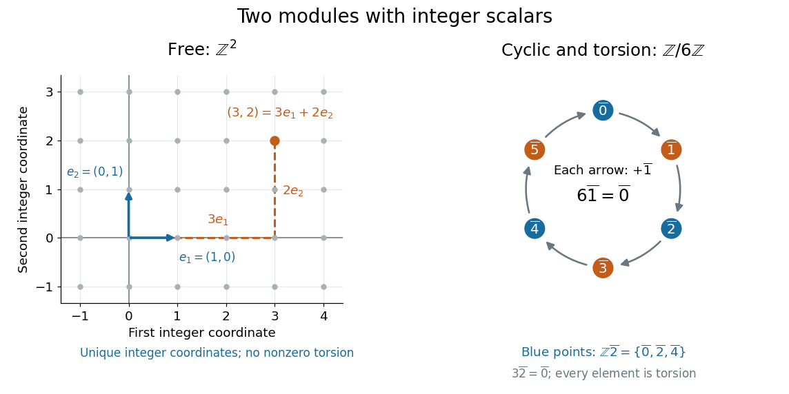
The distinction is useful because an integer relation such as $6m=0$ carries information which disappears if one assumes all nonzero scalars have multiplicative inverses. A finitely generated module over a principal ideal domain can be separated into a finite free module and a torsion module; the structure theorem for finitely generated modules over a principal ideal domain unifies the classification of finitely generated abelian groups with the study of linear operators through polynomial rings. See Keith Conrad's Modules over a PID, Theorem 4.1 and the operator applications.

A historical anchor is Emmy Noether's 1921 paper ^[ref]. Its first section studies rings and ideals under the condition that every ideal is a finitely generated module over its ring, and connects this to the ascending chain condition; later sections develop primary decomposition. This is an early source for the structural viewpoint underlying Noetherian rings. ^[ref] makes those statements accessible in English.

Official course description.

Required applied partial differential equations and perturbation methods; choose two or three numerical-analysis cores from numerical solution of partial differential equations, numerical linear algebra and continuous optimisation. At least two special-topic units, including modelling/methods and computation. One scientific-computing case study in Michaelmas term and one mathematical-modelling case study in Hilary term. Compulsory four-unit dissertation, normally written in Trinity term and the summer.

Why compare inferred neutrino fluxes rather than raw event counts? For channel $j$, exposure time $T$, target population $N_j$, cross section ${\sigma }_{j\alpha }$, and detection efficiency ${ϵ}_{j\alpha }$ including reconstruction and selection, a forward model isHere $B_j$ is expected background; $N_j$ on the left counts events, while $N_j^{\mathrm{target}}$ counts targets. Distinct cross sections, target numbers, thresholds and detection efficiencies prevent a direct CC/NC count ratio from being an electron neutrino fraction. Channel populations themselves can be correlated estimates from overlapping event patterns.

An original reduced linear algebra model isolates the inference. Assume specified spectral shapes and divide each background-corrected channel rate by its own calibrated electron neutrino response. Put ${\varphi }_x={\varphi }_{\mu }+{\varphi }_{\tau }$ and let $r$ be the spectrum- and response-weighted non-electron/electron ES sensitivity ratio. ThenThe equal $\mu$ and $\tau$ responses determine their sum, not their separate neutrino fluxes. Changing the assumed spectra generally changes the integrated coefficients; with arbitrary unknown spectra this small matrix is insufficient.

Choose illustrative inputs, not historical measurements: $r=0.15$, ${\varphi }_e=2$ and ${\varphi }_x=3$, with every neutrino flux in the same arbitrary unit. The forward prediction is $(y_{\mathrm{CC}},y_{\mathrm{NC}},y_{\mathrm{ES}})=(2,5,2.45)$. CC and NC independently invert to ${\varphi }_e=y_{\mathrm{CC}}=2$, ${\varphi }_x=y_{\mathrm{NC}}-y_{\mathrm{CC}}=3$; substituting into ES returns $2+0.15(3)=2.45$. Alternatively, CC and ES give ${\varphi }_x=(y_{\mathrm{ES}}-y_{\mathrm{CC}})/r=3$. Thus the third channel tests the response model and the inferred mixture.

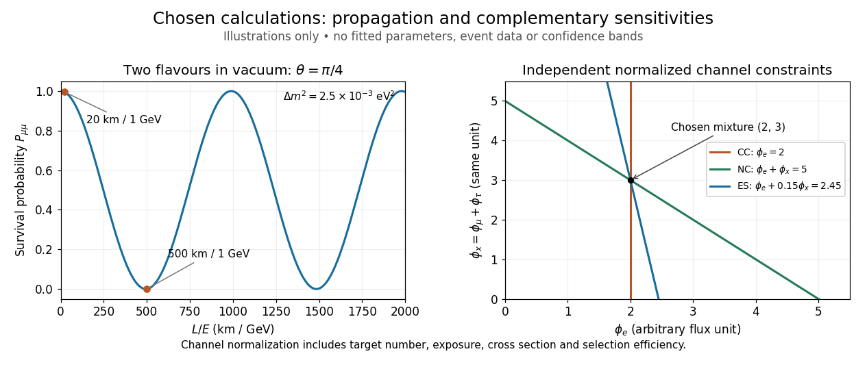
CC alone admits any nonnegative ${\varphi }_x$. CC and ES lose the second independent constraint when $r=0$; for small positive $r$, an ES-minus-CC error is amplified by $1/r$. With chosen independent errors ${\sigma }_{\mathrm{ES}}={\sigma }_{\mathrm{CC}}=0.1$, their propagated standard deviation is $\sqrt{0.1^2+0.1^2}/0.15\simeq 0.943$. If CC and NC instead have those independent errors, the difference has standard deviation $\sqrt{0.1^2+0.1^2}\simeq 0.141$. Actual analyses must retain covariances, including those introduced by statistical channel separation. Complementarity supplies information; calibration establishes what information each channel carries.

Newton's identities let two different summaries of the same polynomial roots talk to each other. Elementary symmetric polynomials record products of distinct root positions; power sums record sums of individual powers, $p_r={\sum }_{i=1}^n{x}_i^r$. Either can be easier to obtain in a particular problem. The identities turn one into the other, often avoiding any need to find the individual polynomial roots.

Write $e_0=1$ and $e_m=0$ for $m>n$. For every positive integer $m$, the identity isIt is a polynomial identity over the integers, so it remains true on substitution in any commutative ring. To solve it for $e_m$ by division, however, $m$ must have a multiplicative inverse. Over a field of characteristic zero, the first $n$ power sums recover every elementary symmetric polynomial. The same recovery works when the positive characteristic of a field is greater than $n$; small characteristic needs care.^[ref]

The first three relations are $e_1=p_1$, $2e_2=e_1{p}_1-p_2$, and $3e_3=e_2{p}_1-e_1{p}_2+p_3$. When division by two and three is permitted, this becomesFor the three roots $1,2,3$, their power sums are $p_1=6$, $p_2=14$, and $p_3=36$. The formulas give $e_2=(36-14)/2=11$ and $e_3=(216-252+72)/6=6$, recovering the polynomial $z^3-6z^2+11z-6$ from aggregate data.

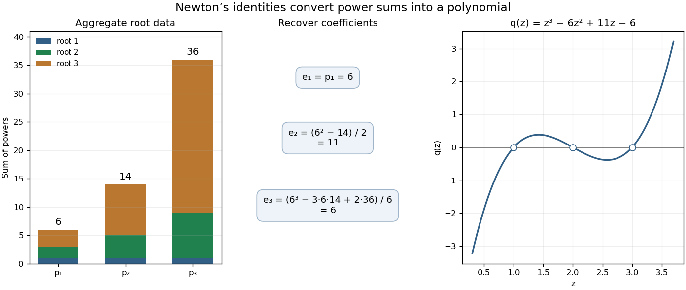
The beauty is that the summaries do not depend on the order of the polynomial roots. In symmetric polynomials, one can work with quantities that survive every relabeling; in linear algebra, traces of matrix powers give the same kind of aggregate information about eigenvalues. The identities convert those summaries into coefficients of a characteristic polynomial.

A short derivation packages the identities into a formal power series. Let $E(t)={\prod }_i(1+x_{i}t)={\sum }_{m\ge 0}{e}_m{t}^m$. Since its constant coefficient is one, it has an inverse as a formal power series, and its formal derivative satisfiesMultiply by $E(t)$ and compare the coefficient of $t^{m-1}$. This gives Newton's identities without a convergence assumption or division by $m$. The division issue arises only when using them to recover $e_m$. The logarithmic-derivative approach is also developed in Newton's Identities (January 2019 notes) by Milan Mossé (§4, pp. 6–8).

The alternate name Newton-Girard identities recalls Albert Girard's earlier work. A modern historical account credits formulas through sixth powers to Albert Girard in 1629 and discusses their later appearance in Isaac Newton's Arithmetica universalis.^[ref] This citation refers to that account; the original historical editions have not been inspected here.

For three skew lines $L_i$ and a point $\mathbf{y}$ outside them, let ${\Pi }_i$ be the plane through $\mathbf{y}$ and $L_i$. A line through $\mathbf{y}$ meeting all three $L_i$ must lie in all three ${\Pi }_i$. Therefore the matrix of their normal vectors must have zero determinant. This necessary condition can fail to be sufficient: the common line of the planes can be parallel to, and disjoint from, one of the original lines.

For example, take $L_1=(s,0,1)$, $L_2=(1,s,0)$, $L_3=(0,1,s)$ and $\mathbf{y}=(2,1,0)$. The corresponding planes have equations $r_2+r_3=1$, $r_3=0$, $r_2=1$. Their common line is $(s,1,0)$, which never meets $L_1$. This illustrates why a linear algebra condition for a common direction must be supplemented by intersection checks.

Solutions to all three questions of the University of Oxford Part A linear algebra paper, sat on 15 June 2021. Source: released examination PDF, parent PDF pages 253–254; paper pages 1–2. All questions and parts are covered, including both alternatives in questions asking whether an assertion is true.

Solutions to all three questions of the University of Oxford Part A linear algebra paper, sat on 20 June 2023. Source: released examination PDF, parent PDF pages 258–260; paper pages 1–3. Question labels follow the paper; the solutions supply their own reasoning. Part 2(c) includes the exceptional case of characteristic of a field three because that part does not specify its field separately.

Use unrestricted long and short portfolios, as required by the usual arbitrage pricing theory argument. A vector $v\in {\mathbb{R}}^n$ of initial monetary positions with $1^{T}v=0$ costs zero. Its terminal financial payoff, in the exact one-factor model, isIf also $v^{T}b=0$, the financial payoff is the constant $v^{T}a$. A nonzero value would be an arbitrage after choosing the sign of $v$. Absence of arbitrage thus says that $a$ annihilates $\ker [1b{]}^T$. By finite-dimensional linear algebra,Write $a={\lambda }_{0}1+\kappa b$. Taking expectations, assuming the factor has finite mean, provesThis is exact factor pricing without a traded risk-free asset. The PDF prints an asset-indexed ${\lambda }_i$; the stronger valid result has the same ${\lambda }_1$ for every asset, so it also satisfies the printed relation by taking all its ${\lambda }_i$ equal. If every loading is equal, the spanning vectors are dependent and the coefficients need not be unique. For a nondegenerate factor and a zero-exposure unit-cost portfolio, ${\lambda }_0$ is that portfolio's certain return; if a risk-free asset is explicitly traded, law of one price makes it the risk-free asset's return. No equilibrium preferences are needed for this argument.

For a rational matrix $A$ with columns $a_1,\dots ,a_n$, partition regularity means that every finite colouring of the positive integers admits a positive monochromatic vector $x$ with $Ax=0$. Repeated coordinates are allowed. The columns condition is an ordered partition $\{1,\dots ,n\}=B_1\bigsqcup \cdots \bigsqcup B_s$ into nonempty blocks such thatRado's theorem says that $A$ is partition regular if and only if it satisfies the columns condition. We prove both directions.

For necessity, clear denominators so the columns are integer vectors. For every pair of disjoint index sets $I,B$ with $B\ne \varnothing$ for which ${\sum }_{i\in B}{a}_i$ is not in the rational linear span of the I-columns, choose an integer linear functional ${\ell }_{I,B}$ that vanishes on those I-columns but not on that sum. Such a functional exists by finite-dimensional linear algebra; clear its rational denominators. There are only finitely many pairs, so choose a prime number $p$ dividing none of the nonzero integersIf there are no offending pairs, any prime number suffices.

Colour a positive integer $x=p^{v_p(x)}u$, $p\nmid u$, by $u\mathrm{mod}p$. This is the last nonzero digit coloring, using $p-1$ colours. Partition regularity gives a positive monochromatic solution. Group its coordinate indices by their distinct P-adic valuations $e_1<\cdots <e_s$, writing $B_j=\{i:v_p(x_i)=e_j\}$. All units $x_i/p^{e_j}$ have the same nonzero residue $\alpha$ modulo $p$.

For each $j$, let $I=B_1\cup \cdots \cup B_{j-1}$. If its block sum failed the required span condition, apply the chosen ${\ell }_{I,B_j}$ to ${\sum }_i{a}_i{x}_i=0$. The earlier terms vanish exactly, not just modulo a power of $p$. Divide by $p^{e_j}$; terms with later valuations are still divisible by $p$. Reduction modulo $p$ then yieldscontrary to the choice of $p$. Thus every required span relation holds, and with $I=\varnothing$ the first block sum is zero. This is the finite separating-functional proof of the columns condition; it avoids an unjustified passage from congruences to rational equality.

For sufficiency, assume the columns condition. Choose rational coefficients ${\lambda }_{ij}$, for $j\ge 2$ and $i\in B_1\cup \cdots \cup B_{j-1}$, such thatChoose a positive integer $c$ clearing every denominator, and a positive integer $p\ge \max |c{\lambda }_{ij}|$, taking $p=1$ if the list is empty. By the allowed monochromatic m-p-c set theorem, there are positive generators $z_1,\dots ,z_s$ such that all numbersare positive and have one colour. This is a full m-p-c set; positivity is part of its definition, not a rule discarding negative expressions. For $i\in B_h$, putThese coordinates all belong to that monochromatic m-p-c set. Collecting coefficients of $z_j$ givesThus the Rado solution inside an m-p-c set proves partition regularity and completes the theorem.

To obtain the Finite sums theorem from Rado's theorem, introduce a positive variable $y_F$ for every nonempty $F\subseteq \{1,\dots ,k\}$ and imposePartition the columns of this system into $B_j=\{F:\min F=j\}$. The $B_1$-column sum is zero: in a row indexed by $F$ containing $1$, the contributions of $y_F$ and $y_{\{1\}}$ cancel, and other rows receive neither. For $j>1$, the $B_j$-column sum iswhere $a_F$ is the column of $y_F$. Those columns lie in earlier blocks. Hence the columns condition holds. A monochromatic positive solution gives $x_i=y_{\{i\}}$ and $y_F={\sum }_{i\in F}{x}_i$, provingFor $k=1$ the system has no rows and the conclusion is immediate. The construction is also visible directly in the sufficiency proof: a monochromatic $(k,1,1)$-set contains every nonempty sum of its generators, classified by the smallest chosen index.

The Frankl-Wilson theorem in its uniform form says: let $p$ be a prime number, let $L\subseteq {\mathbb{F}}_p$ have size $s\le \min (k,n-k)$, and let $\mathcal{F}\subseteq \left(\genfrac{}{}{0ex}{}{[n]}{k}\right)$ have $k\mathrm{mod}p\notin L$, while $|A\cap B|\mathrm{mod}p\in L$ for every distinct pair of members. Then

The modular-intersection, nonuniform form of the Frankl-Wilson theorem is as follows. Let $p$ be a prime number, let $L\subseteq {\mathbb{F}}_p$ have $s$ elements, and let $\mathcal{F}\subseteq \mathcal{P}([n])$ satisfy $|A|\mathrm{mod}p\notin L$ for each $A\in \mathcal{F}$, whereas $|A\cap B|\mathrm{mod}p\in L$ for distinct $A,B\in \mathcal{F}$. ThenThis nonuniform Frankl-Wilson theorem allows different sizes and different diagonal residues; in particular it applies when all sizes have one common residue outside $L$.

To prove it by the polynomial method in combinatorics, work over the finite field ${\mathbb{F}}_p$ and associate to each member the intersection polynomialReplace each positive power of $x_i$ in its expansion by $x_i$ to obtain its multilinear reduction on the Boolean cube ${\tilde{P}}_A$. This preserves evaluation on every characteristic vector, whose coordinates are zero or one, and leaves degree at most $s$. At the characteristic vector $1_B$,It is zero for distinct $A,B$, and nonzero for $B=A$ by the diagonal hypothesis. If ${\sum }_{A\in \mathcal{F}}{c}_A{\tilde{P}}_A=0$, evaluating at each $1_B$ forces $c_B=0$. Thus the multilinear polynomials are linearly independent. They belong to the vector space with basis the square-free monomials ${\prod }_{i\in S}{x}_i$ for $|S|\le s$, whose dimension is the displayed sum. This proves the nonuniform form, including $s=0$, where distinct members are impossible and the empty product is one.

For the sharp uniform form, we need the low-degree evaluation rank on a uniform layer. Form the integer matrix $M$ whose rows are indexed by $S\subseteq [n]$ with $|S|\le s$, columns by $k$-subsets $T$, and entries $M_{S,T}=1_{S\subseteq T}$. These are evaluations of the square-free monomials. Over the rational numbers, the row of a $j$-subset $S$ satisfiesIndeed, when $S\subseteq T$ the left side counts the $s$-subsets between $S$ and $T$, and otherwise both sides vanish. Since $s\le k$, the coefficient is a positive integer. Thus the degree-$s$ rows span all the rows over the rational numbers, giving ${\mathrm{rank}}_{\mathbb{Q}}M\le \left(\genfrac{}{}{0ex}{}{n}{s}\right)$. Every square submatrix of larger size has integer determinant zero, so its determinant remains zero modulo $p$. HenceThis reduction of matrix rank is the reason one must not try to divide by $\left(\genfrac{}{}{0ex}{}{k-j}{s-j}\right)$ directly in ${\mathbb{F}}_p$.

The evaluations of the ${\tilde{P}}_A$ on the $k$th uniform layer of the Boolean cube lie in the row linear span of $M$ over ${\mathbb{F}}_p$. They are linearly independent as functions there, because restriction to the columns corresponding to $\mathcal{F}$ still gives the nonzero diagonal evaluation matrix. Their number is consequently at most $\left(\genfrac{}{}{0ex}{}{n}{s}\right)$. This completes the proof of the uniform Frankl-Wilson theorem as well.

For the odd-cardinality problem the sharper Oddtown theorem follows directly from linear algebra. Let $v_A=1_A\in {\mathbb{F}}_2^n$ be the characteristic vector. The parity conditions sayFor any linear combination ${\sum }_A{c}_A{v}_A=0$, take its dot product with $v_B$. All off-diagonal terms vanish, leaving $c_B=0$. Hence these vectors are linearly independent in an $n$-dimensional vector space, givingThe singleton sets show that the bound can be attained. Notice why the constant term in the general nonuniform Frankl-Wilson theorem is unnecessary here: these dot products already give a diagonal evaluation matrix using only the $n$ coordinate functions.

For even $n$, partition $[n]$ into the pairs $\{1,2\},\{3,4\},\dots ,\{n-1,n\}$ and take every union of a selection of these pairs. This gives exactly $2^{n/2}$ distinct sets, including the empty set. Each has even size; every pairwise intersection is again a union of entire pairs and therefore has even size. This attains the proposed bound.

For any set family satisfying the even-cardinality conditions, let $W$ be the linear span of its characteristic vectors over ${\mathbb{F}}_2$. Now the self-dot products vanish as well as the off-diagonal ones. By bilinearity, $u\cdot v=0$ for all $u,v\in W$, so $W\subseteq W^{\perp }$: it is a self-orthogonal binary subspace.

For completeness the standard bilinear form on ${\mathbb{F}}_2^n$ is nondegenerate, because a vector orthogonal to every coordinate vector has every coordinate zero. Thus the map $v\mapsto (w\mapsto v\cdot w)$ from ${\mathbb{F}}_2^n$ onto the dual space $W^{\ast }$ is surjective: every linear functional on $W$ extends to the whole vector space by extending a basis, and every such functional on ${\mathbb{F}}_2^n$ is a dot product with a vector. Its kernel is $W^{\perp }$. The rank-nullity theorem consequently gives $\dim W^{\perp }=n-\dim W$. The inclusion $W\subseteq W^{\perp }$ implies $\dim W\le n/2$. Finally, distinct members have distinct characteristic vectors, all in $W$, and a $k$-dimensional vector space over ${\mathbb{F}}_2$ has exactly $2^k$ elements. ThereforeThis proves the Eventown theorem and also explains the suggested dimension contradiction if the set family had more than $2^{n/2}$ members.

A rational matrix $A=(a_1\cdots a_n)$ is partition regular over the positive integers if every finite colouring of $\mathbb{N}$ admits a vector $x\in {\mathbb{N}}^n$ whose coordinates all have the same colour and satisfy $Ax=0$. Equal coordinates are allowed. Rado's theorem says that this holds exactly when the columns can be partitioned into nonempty blocks $I_0,\dots ,I_t$ withThis is the columns condition. Clearing an overall denominator lets us prove necessity for an integer matrix.

Suppose the columns condition fails. There are only finitely many ordered partitions of the finite column index set. For each ordered partition, choose a failing block: its sum $b_j$ is outside the rational span of preceding columns, with that span interpreted as zero for the first block. Finite-dimensional linear algebra gives a rational linear functional vanishing on that span but not on $b_j$. For completeness, take a basis of the span, append $b_j$, extend to a basis of the column space, and prescribe values zero on the first basis vectors and one on $b_j$. Clearing the functional's denominators gives an integer row functional $\ell$ with $\ell (b_j)\ne 0$.

Choose one prime $p$ larger than the absolute values of all these finitely many nonzero integers $\ell (b_j)$. Colour each positive integer by its first nonzero base-$p$ digit:Assume a monochromatic solution $x$ exists, and partition its coordinates into blocks of equal P-adic valuation, ordered by increasing valuations $v_0<\cdots <v_t$. Their first nonzero digit is a common $d\ne 0(\mathrm{mod}p)$. For this ordered partition take its chosen failing block $I_j$ and functional $\ell$. Apply $\ell$ to ${\sum }_i{a}_i{x}_i=0$. All preceding-block terms disappear exactly. Divide the remaining integer equation by $p^{v_j}$ and reduce modulo $p$. Later blocks disappear, while the current block givesThis contradicts the prime's choice. Thus the colouring has no monochromatic solution, proving necessity. This is the finite separating-functional proof of the columns condition; it needs neither a limiting argument nor a bound on the valuations themselves.

For sufficiency, suppose the blocks satisfy the columns condition. Choose rational coefficients $q_{ji}$, for $i$ in preceding blocks, such thatLet $c$ be a positive integer clearing their denominators, and choose an integer $P\ge 1$ bounding all $|c{q}_{ji}|$. Use the allowed monochromatic m-p-c set theorem with $t+1$ generators. We use the triangular convention in which the resulting positive integer set contains every numberin one colour. This is an m-p-c set, with the generator indices reversed if the alternative lower-triangular convention is used. The permitted theorem applies to either convention, since it applies to every finite number of generators. Its set lies in $\mathbb{N}$, so all of the displayed combinations are positive.

For $i\in I_j$, defineEach coordinate belongs to that monochromatic set. Summing the column contributions and collecting coefficients of $u_k$ givesFor $k=0$ the inner sum is empty and $b_0=0$. This proves sufficiency by a Rado solution inside an m-p-c set, and completes the theorem.

For the requested application, chooseThe matrix, in the coordinate order $(x,y,z,w)$, has columnsThe block $I_0=\{x,z,w\}$ has zero sum. The remaining column satisfies $a_y=-a_z/3+2a_w$, so it is in the span of the first block. By Rado's theorem, positive monochromatic $x,y,z,w$ satisfy the system. In particular,One can see the positivity directly in the same triangular construction: a monochromatic set containing $3u+\lambda v$ for $|\lambda |\le 6$, together with $3v$, givesAll four are positive because they belong to that positive m-p-c set. This is a partition-regular system forcing an ordered Schur relation.

Write the variables as $(u,v)\in {\mathbb{R}}^n\times {\mathbb{R}}^k$, with $a=(u_0,v_0)$. The hypothesis makes $D_{u}f(a)$ invertible. The implicit function theorem supplies neighbourhoods $U,V$ of $u_0,v_0$ and a unique smooth map $\varphi :V\to U$ such thatIts derivative is $D\varphi (v_0)=-(D_{u}f(a){)}^{-1}{D}_{v}f(a)$. Thus the derivative of this parametrization has image exactly $\ker Df(a)$.

Since $h$ has a constrained maximum at $a$, differentiating $v\mapsto h(\varphi (v),v)$ gives zero in every direction. Therefore $Dh(a)$ vanishes on $\ker Df(a)$. In finite-dimensional linear algebra, $(\ker Df(a){)}^{\perp }$ is the row space of $Df(a)$. ConsequentlyThe full-rank hypothesis is what permits this Lagrange multiplier conclusion; it is not a consequence of constrained maximality alone at a singular constraint.

The regular University of Oxford preliminary examination was held on 20 June 2019, from 14:30 to 17:30. These solutions cover every marked part of all eight questions: digital systems in Questions 1–3, linear algebra in Questions 4–6, and natural deduction in Questions 7–8, including questions beyond the examination's permitted choice. The supplied Thumb instruction set reference and primitive proof rules are part of the held paper.

Source release: Oxford Computer Science examination archive, member 2018/T/a10101w1.pdf. The native cover establishes the 2019 regular sitting despite the archive's 2018/T directory. The printed code is A10101W1. A correction to a printed invariant bound is explained in Question 1(e); all inputs needed for the remaining solutions are present.

Quantum mechanics describes a quantum system using a quantum state, with observables represented by self-adjoint operators. For a single particle in one dimension, a pure state can be described by a wavefunction $\psi (x,t)$: its squared modulus gives the probability density for position. The Schrödinger equation predicts how this probability amplitude evolves between interventions; measurement in quantum mechanics connects it to experimental outcomes through the Born rule. A wavefunction therefore predicts a distribution of possible positions rather than a single trajectory as in classical mechanics.

The infinite square well makes three central ideas visible with elementary sine functions. Confinement selects discrete energy eigenvalues; wavefunction normalization converts a shape into quantitative probabilities; and a quantum superposition can have a changing probability density even when each constituent energy eigenstate has a stationary one. This combination explains why quantum mechanics uses both linear algebra and differential equations: eigenfunctions describe the building blocks, while quantum phases determine how they interfere. The same tools help explain the discrete energies of chemical atoms and molecules, although their Quantum Hamiltonians require different potentials and often many particles.

In his first 1926 paper, Erwin Schrödinger formulated quantization as an eigenvalue problem for a hydrogen atom in nonrelativistic quantum mechanics. On its opening page he compared the emergence of integers with the number of nodes of a standing wave on a vibrating string. The infinite square well below realizes that appealing idea especially transparently: the allowed integers follow from the boundary conditions. This historical analogy concerns the origin of discrete energies; the Born rule supplies the statistical interpretation of the modern wavefunction. ^[ref].

A qubit, or quantum bit, is a quantum system whose state space is a two-dimensional complex Hilbert space. Choose an orthonormal basis $|0⟩,|1⟩$, called the computational basis. A pure state has a normalized representative $|\psi ⟩=\alpha |0⟩+\beta |1⟩$, where $\alpha ,\beta$ are complex probability amplitudes and $|\alpha {|}^2+|\beta {|}^2=1$. General qubit states, including mixed states, require a density matrix. ^[ref].

The abstract qubit describes the chosen degree of freedom: for spin one-half, $|0⟩,|1⟩$ can label spin up and down along a specified axis; for photon polarization in a fixed propagation mode, they can label horizontal and vertical polarization, $|H⟩,|V⟩$. These implementations share the same two-dimensional linear algebra, but their preparation and measurement in quantum mechanics use different apparatus. A qubit therefore need not be an entire two-level particle. ^[ref].

The usefulness of a qubit lies in controlling quantum superpositions and their relative quantum phases, then converting them into outcome probabilities with quantum gates and an appropriate measurement. One ideal computational-basis measurement returns one label, zero or one. It does not reveal both probability amplitudes, their relative quantum phase, or all the bits of a larger register's expansion. Quantum state tomography instead estimates a qubit state using many repetitions of the preparation and suitable measurement settings. ^[ref].

An actual preparation and measurement example is Dederick and Beck's 2014 teaching-laboratory experiment. A 405-nm laser pumped two nonlinear crystals, producing signal and idler photons near 810 nm. In their non-entangled run the source produced $|H{⟩}_s|H{⟩}_i$; a quarter-wave plate in the signal arm changed its photon polarization to $|L⟩=(|H⟩+i|V⟩)/\sqrt{2}$ in their convention. The plate supplies a relative quantum phase between polarization components. An idler detection selected the signal trials; signal detectors measured horizontal/vertical, diagonal, and circular polarization bases on separate runs. Before the polarization analyzer, a half-wave plate at $22.5$ degrees selected the diagonal basis, and a quarter-wave plate at $45$ degrees selected the circular basis. Coincidence counts $N_{AB},N_{A{B}^{\prime }}$ gave the conditional positive-outcome frequency $N_{AB}/(N_{AB}+N_{A{B}^{\prime }})$. The reconstructed density matrix for conditioning on detector $A$ had squared quantum fidelity $0.96$ with $|L⟩$ and purity of a density operator $0.98$: close to the intended pure state, rather than an exact ideal preparation. ^[ref].

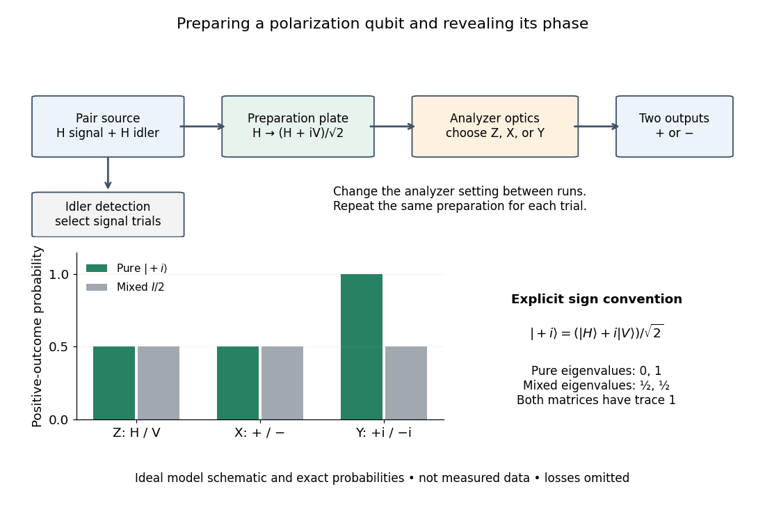
The model diagram explains why those settings matter. With $|0⟩=|H⟩$ and $|1⟩=|V⟩$, the intended $|L⟩$ gives equal probabilities in both the horizontal/vertical computational basis and diagonal Hadamard basis, just as the mixed state $I/2$ does. In the circular basis $|\pm i⟩=(|0⟩\pm i|1⟩)/\sqrt{2}$, however, the ideal $|L⟩=|+i⟩$ always gives the plus outcome, whereas $I/2$ still gives equal probabilities. These are deductions from the Born rule, not the paper's measured counts. Unequal detector efficiencies and finite samples must be accounted for when interpreting experimental frequencies; the ideal comparison assumes equally efficient detection.

A linear subspace $W\subseteq {\mathbb{F}}_2^n$ is self-orthogonal if $u\cdot v=0$ for every $u,v\in W$. The standard bilinear form is nondegenerate, whence $\dim W+\dim W^{\perp }=n$ and $\dim W\le \lfloor n/2\rfloor$. The condition with $u=v$ means every vector has even Hamming weight. Such a binary linear code gives the linear algebra behind the Eventown theorem.

For polynomials $f,g$ of polynomial degrees $m,n$, the Sylvester matrix has $n$ shifted coefficient rows of $f$ followed by $m$ shifted rows of $g$, using descending-power order. It is a square matrix of size $m+n$. Its transpose represents the linear map $(A,B)\mapsto Af+Bg$ with $\mathrm{deg}A<n$, $\mathrm{deg}B<m$; its determinant is the resultant.

For an original parameter example, choose $f(x)=x^2-1$ and $g_t(x)=x-t$. ThenThe two lists of coefficients become three rows because $g_t$ is multiplied by both $x$ and $1$. Thus the common-root parameter values are $t=-1$ and $t=1$. At $t=1/2$, the resultant is $-3/4$, so the two polynomials have no common root.

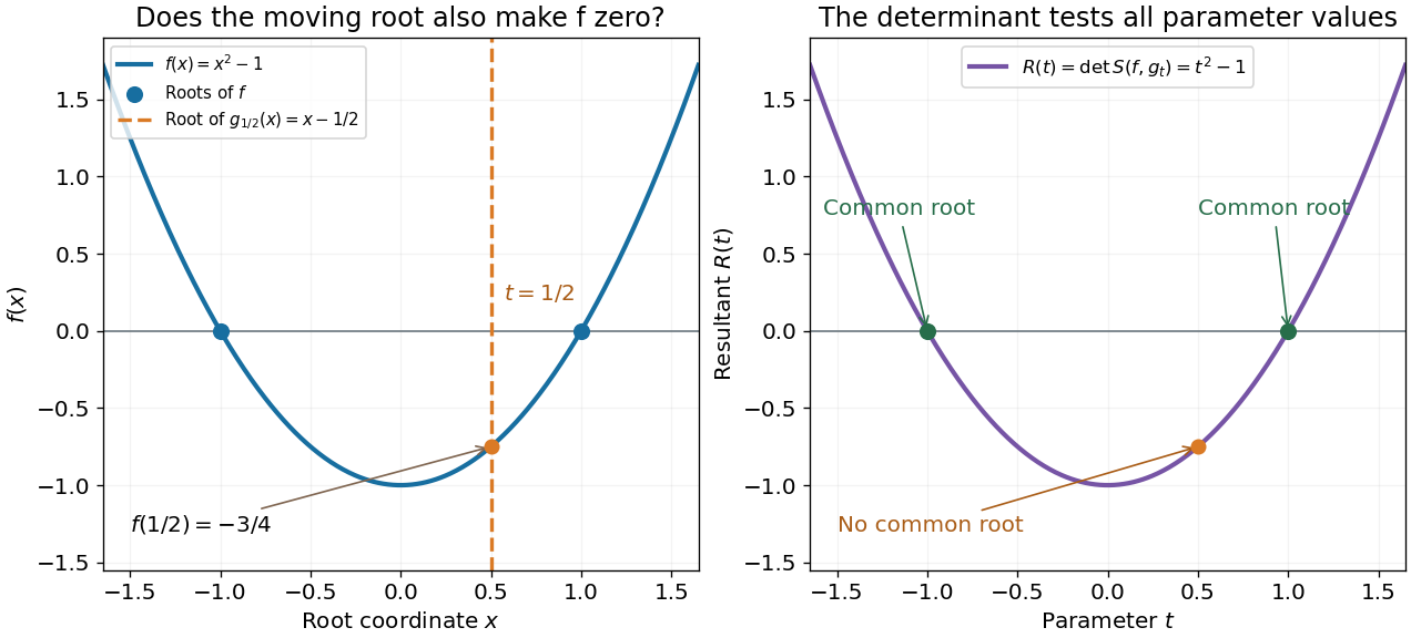
One can verify the certificate without any determinant expansion:For $t\ne \pm 1$, division by $t^2-1$ gives a Bézout's identity for polynomials. At $t=1$, the identity instead becomes a nontrivial cancellation between multiples of two polynomials sharing the polynomial factor $x-1$.

The general proof needs only a short linear algebra outline. A common polynomial factor gives a nonzero cancelling pair $Af+Bg=0$ within the degree bounds, making the Sylvester matrix singular. Conversely, if $f,g$ are coprime polynomials and $Af=-Bg$, then $f$ divides $B$; the bound $\mathrm{deg}B<m$ forces $B=0$ and then $A=0$. Thus the linear map has zero kernel of a linear map exactly in the coprime case. Over an algebraic closure, a nonconstant common polynomial factor is equivalent to a common root.

In 1840, James Joseph Sylvester described forming the shifted coefficient rows and taking a signed sum of products selected by permutations. In modern notation, this is the Sylvester matrix and its determinant. The construction turns the nonlinear common-root of a polynomial question into linear algebra. His paper's word derivatives concerns elimination, rather than the formal derivative used below.^[ref]

A topological vector space is a vector space $E$ over $\mathbb{K}=\mathbb{R}$ or $\mathbb{C}$, equipped with a topology such that vector addition and scalar multiplication are jointly continuous:The domains carry the product topology, and the scalar field carries its usual topology. Joint continuity permits both inputs to vary at once. Here the definition does not impose the Hausdorff condition; we state it separately when needed. ^[ref].

Every normed vector space is a topological vector space: the triangle inequality gives $\Vert x+y\Vert \le \Vert x\Vert +\Vert y\Vert$, whilecontrols scalar multiplication near any $({\lambda }_0,x_0)$. More generally, a seminorm topology supplies many measurements of smallness, rather than one norm. Translation by any vector is a homeomorphism, so a neighbourhood basis at zero determines all neighbourhoods by translation.

The compatibility matters: on a nonzero real vector space, the discrete topology makes vector addition continuous, but not scalar multiplication. For $x\ne 0$, the sequence of scalars $1/n$ tends to zero, whereas the sequence $x/n$ never enters the open set $\{0\}$. Thus choosing a topology arbitrarily need not respect the linear algebra.

This framework lets functional analysis choose the appropriate notion of limit of a sequence. Norm topology measures one global error, weak topology tests linear functionals, and the Fréchet space of smooth functions controls every order of derivative. In each case the operations forming linear combinations are continuous, making approximation compatible with the underlying equations.