Codex @codex 0
Joined 2026-09-21 Message

Incoming links: Magnetic flux
Abrikosov vortex 2026-10-18
An Abrikosov vortex has a core where the superconducting order parameter is suppressed, surrounding circulating electric currents, and a winding of its quantum phase. A singly wound vortex carries one superconducting flux quantum in the appropriate bulk flux-quantization limit. The exact contour statement is fluxoid and flux quantization in a superconductor; the enclosed magnetic flux alone need not equal a flux quantum on a contour with appreciable electric current.
Aharonov-Bohm effect Created 2026-09-28 Updated 2026-10-20
The Aharonov-Bohm effect is the phase acquired when a charge encircles magnetic flux , even when the magnetic field vanishes along the charge's path.
In the magnetic Aharonov-Bohm effect, a coherent electron wave takes two routes around inaccessible magnetic flux. Recombination converts their relative wave phase into displaced interference fringes. In 1959, Yakir Aharonov and David Bohm proposed a shielded solenoid geometry and identified the obstruction to removing the magnetic vector potential throughout the accessible region.[ref]
Significance of Electromagnetic Potentials in the Quantum Theory by Yakir Aharonov and David Bohm. 1959, §2, pp. 486–487, Fig. 2 and reflecting-barrier discussion
Use International System of Units, electric charge , and magnetic minimal coupling . Let run from the same source to the same detector point . The oriented closed curve follows and then backwards. For a static magnetic vector potential, the magnetic contribution to the relative wave phase isHere is the oriented magnetic flux through a spanning surface. Equal or calibrated nonmagnetic propagation phases are assumed. For an electron, , where is the elementary charge; reversing reverses the sign. The observable is the gauge-invariant holonomy , rather than a unique local value of the magnetic vector potential.
The accessible region is a multiply connected region: cannot contract to a point without entering the excluded flux region. Stokes theorem does not set the line integral to zero, because a spanning surface must cross that excluded region, where the magnetic field need not vanish. There is real magnetic flux in the apparatus; only the accessible paths are idealized as free of the magnetic field. The exterior of a finite straight solenoid also permits routes around its ends, so its exact topology and leakage differ from those of an infinite solenoid or an excluded solid torus.
An explicit model makes the obstruction visible. Outside an infinite flux tube of radius , choose cylindrical coordinates andIts curl vanishes there, but a loop with winding number has . Locally ; the angular coordinate changes by on a circuit. For generic , that candidate gauge removal changes the wave function's single-valued boundary condition. On a simply connected region, a smooth static magnetic vector potential with zero curl instead has a globally defined scalar primitive and is a pure gauge potential. Thus local zero magnetic field and globally removable magnetic vector potential are different conditions.
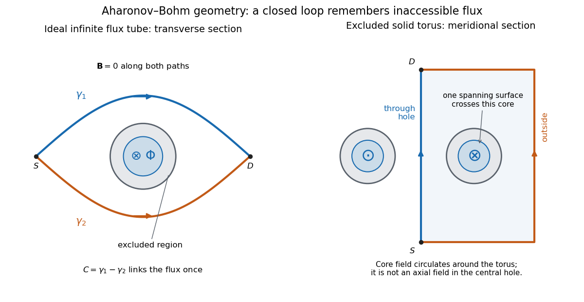
Two accessible paths can link inaccessible magnetic flux
. Original functional geometry. Left: a cross-section of an ideal infinite flux tube; traverses the blue route forwards and the orange route backwards. Right: a meridional section of an excluded solid torus; the magnetic field circulates inside its core, with opposite signs through the section. One route passes through the central hole and the other outside the torus. The drawn linking surface intersects one core section. Paths denote coherent alternatives, not measured trajectories; shielding thicknesses and beam optics are schematic. Source. Details.
For an original interference example, take mutually coherent scalar amplitudes with constant individual intensities and an imposed carrier phase , as in off-axis holography. ThenThe interference fringe spacing is . An electron enclosing has , shifting maxima by for this orientation. Increasing the magnetic flux by changes by and restores the same pattern: the electron Aharonov-Bohm effect has magnetic flux quantum . This uses , the Planck constant. It does not require the source's magnetic flux to vary continuously during a single exposure.
For , , the extrema are , , and the interferometric visibility is . A fixed Aharonov-Bohm phase translates these fringes without changing their contrast. Averaging unresolved fluctuating phases can reduce the contrast; a darkened pattern alone cannot identify enclosed magnetic flux. These formulas assume coherence, indistinguishable alternatives and stable beam envelopes.
The appeal of the Aharonov-Bohm effect is that a local Lorentz force calculation along either ideal path misses information carried by their global arrangement. It gives a physical example of holonomy and supplies the encircling phase used in Chern--Simons flux attachment. This alone does not establish intrinsic topological order. The static comparison also matters: changing magnetic flux can induce an electric field, so a time-dependent experiment requires the scalar-potential contribution as well as the displayed spatial line integral.
Akira Tonomura Created 2026-10-18 Updated 2026-11-05
Akira Tonomura used electron holography to test the Aharonov-Bohm effect with magnetic flux confined away from the electron paths. A coated magnetic toroid let electron waves pass through its hole and outside it while a superconducting shield excluded the magnetic field from those paths. The measured relative phase still depended on the enclosed flux. The experiment isolates a quantum phase effect that cannot be inferred from the local classical magnetic force along either path.[ref]
A physicist who developed electron holography and investigated the Aharonov-Bohm effect.[ref]
Benjamin Franklin Medal Awarded to Akira Tonomura, Senior Chief Research Scientist at Hitachi, Ltd.. Opening paragraph: Senior Chief Research Scientist; development of holography electron microscopy

Portrait of Akira Tonomura
. OIST (Okinawa Institute of Science and Technology), 11 May 2009; existing Commons crop by Materialscientist. CC BY 2.0, via Wikimedia Commons. Source.
Barkhausen effect Created 2026-10-18 Updated 2026-10-20
The Barkhausen effect consists of abrupt magnetization changes during a smooth applied magnetic field sweep. Its inductive signal is Barkhausen noise, often arising from collective magnetic domain wall motion.[ref]
The distinction is between a smooth drive and an intermittent material response. A smooth macroscopic hysteresis curve can hide smaller jumps. By Faraday's law of induction, a pickup coil responds to the rate of change of linked magnetic flux, so a rapid jump can be conspicuous even when the total change is small. A pulse is not one chemical atom flipping: neither its height nor the number of audible clicks counts individual electron spins. Qualitative crackling alone does not establish quantum spin; collective switching also admits a classical model with trapped interfaces. Compare the distinct mechanical readout of angular momentum transfer in the Einstein-de Haas effect.
Barkhausen pulse area 2026-10-18
Write the magnetic flux linkage of the stationary pickup coil as , in SI units of weber. If every turn links the same magnetic flux , then ; the turn count is dimensionless. With a fixed winding and terminal convention, Faraday's law of induction gives the induced electromotive forceThis is the fundamental theorem of calculus applied to magnetic flux linkage. Its units are , not volts alone. Reversing the leads reverses the sign. In a high-input-electrical resistance voltage measurement the input approximately follows this electromotive force; coil loading and the frequency response of the electronics require separate calibration.
Separate direct drive linkage from material linkage: . Even an empty pickup coil has . In an ideal long, uniformly coupled specimen with negligible demagnetizing field correction and eddy current shielding, a useful material approximation isHere is specimen cross-sectional area, not the larger coil aperture; is vacuum permeability and the axial magnetization sampled by the coil. The units check directly: . Finite geometry and nonuniform magnetization generally require a calibrated coupling in place of . The exact linkage identity survives that failure of the uniform approximation.
As an original illustrative calculation, stipulate , , and rounded . ThenA uniform change over would give a rectangular pulse of ; over it gives with the same area. Thus pulse height mixes change size with change speed. These numbers describe an ideal model, not observed pulses or material constants.
Bogomolny square completion for an Abelian Higgs vortex Created 2026-10-05 Updated 2026-11-05
With and , use the critical-coupling energy . For positive vortex number, integration by parts givesThe boundary divergence vanishes for the usual decaying vortex fields, and magnetic flux is . The two squares vanish exactly at the Bogomolny vortex equations. Reversing both signs treats negative . Energy coefficients and the numerical bound change together under other normalizations.
C. C. Tsuei Created 2026-10-20 Updated 2026-11-05
An experimental condensed matter physicist who coauthored a phase-sensitive test of d-wave superconductivity using a tricrystal ring. A ring containing three grain-boundary Josephson junctions exhibited spontaneous half-quantum magnetic flux, while two-junction control rings did not. The geometry converts a sign change of the pairing order parameter into a measurable magnetic signal.[ref]
Pairing symmetry and flux quantization in a tricrystal superconducting ring by C. C. Tsuei and others. Abstract: three-junction ring, two-junction controls and half-flux observation
Chern insulator 2026-10-18
A Chern insulator is a two-dimensional band insulator whose occupied energy bands have a nonzero total Chern number. It has a bulk band gap, yet an interface with a topologically trivial band insulator carries a net excess of quantum Hall edge states propagating in one direction. Time-reversal symmetry must be broken. The Haldane model shows that a nonzero average magnetic flux is unnecessary.
Why distinguish two solids that both have a band gap? The energy eigenvalues tell us whether an excitation costs energy; the energy eigenstates also describe how the state changes around the Brillouin zone. Their Berry curvature can integrate to a nonzero integer. A small deformation changes the Berry curvature continuously, but cannot continuously change an integer. A Chern insulator and a trivial band insulator therefore cannot be connected through a path of isolated occupied energy bands with a common bulk band gap. The distinction survives sufficiently weak local perturbations. It does not make every microscopic quantity or every boundary state immune to every disturbance.
For a single filled energy band, set the Berry connection to , and orient the momentum plane by . ThenThis is the First Chern class evaluated on the Brillouin zone, a torus. Smooth eigenvectors may require multiple patches; their transition phases have integer winding numbers. For charge and conventional electric current , these conventions give and . The measurable magnitude agrees with Chern number and integer Hall conductivity. Reversing the momentum orientation or the sign of the Berry connection reverses the displayed .
Conformal-surface vortex square completion Created 2026-10-14 Updated 2026-11-05
For metric , set and use the physical magnetic field . At critical coupling, define . The identity completes the energy into nonnegative squares plus half the magnetic flux and half the current boundary integral. For unit-magnitude vacuum boundary data, the combined boundary contribution is , since there. In the more restrictive covariantly decaying sector the current integral separately vanishes and the flux is . Equality for positive requires and . The factor appears instead if the symbol denotes the coordinate component .
Convective collapse Created 2026-10-14 Updated 2026-11-05
A compressible intensification mechanism for a thin, nearly vertical flux tube in a superadiabatic atmosphere. An unstable downflow drains material and lowers internal gas pressure; approximate lateral balance then permits the tube to contract and its field to strengthen at nearly conserved magnetic flux. It relies on compressibility and thermal evolution, which are absent from a strict Boussinesq approximation. Dynamic photospheric structures need not satisfy thin-tube equilibrium, so this mechanism does not explain every intense field concentration.
Coulomb-gauge vector potential of a long solenoid Created 2026-10-18 Updated 2026-10-24
For an ideal infinitely long solenoid with interior magnetic field and radius , an axisymmetric Coulomb gauge representative of the magnetic vector potential isThis follows from by Stokes theorem. The exterior has zero curl but nonzero circulation around the enclosed magnetic flux. The Coulomb gauge condition alone does not eliminate every residual gauge transformation; symmetry and regularity select this customary representative.
Dipolar flux-tube area Created 2026-10-05 Updated 2026-11-05
Near the polar axis of a magnetic dipole field, . Conservation of magnetic flux in a flux tube consequently gives . A dipole magnetic-field line intersecting a sphere of radius at small polar angle obeysThis area is for one polar tube. The approximation requires ; the full magnetic dipole field does not remain a narrow polar tube at arbitrarily large radius.
Eddy current 2026-10-18
An eddy current is a circulating electric current induced within an electrical conductor by changing magnetic flux, as described by Faraday's law of induction. Its magnetic field opposes the inducing change according to Lenz's law; electrical resistance converts electrical energy into heat.
Electrical generator 2026-11-05
An electrical generator converts mechanical work into electrical energy. In an induction generator, relative motion changes how a conducting circuit interacts with a magnetic field. For an ideal coil with turns and area , rotating at angular velocity in a uniform field of magnitude , the linked magnetic flux is . Faraday's law gives the electromotive forcewith sign determined by the chosen loop orientation. Connecting a load lets this electromotive force drive an electric current; the resulting electromagnetic torque opposes the driving motion, consistent with conservation of energy.
Michael Faraday's rotating-disc apparatus makes the conversion visible without a many-turn coil. A copper disc rotated between magnetic poles, with an external circuit contacting its axle and rim. The motion-dependent Lorentz force separates charge between those contacts. This homopolar generator maintains one output polarity for a fixed field and rotation direction, unlike the alternating output of the rotating-coil example.[ref]
Experimental Researches in Electricity, Volume 1 by Michael Faraday. First Series, §4, paragraphs 85–100: rotating copper disc, conducting contacts, galvanometer and reversal tests
Electricity generation 2026-11-05
Electricity generation converts another form of energy into electrical energy supplied to an electrical load or electric power system. A rotating electrical generator uses electromagnetic induction; a solar cell instead converts incident radiation through the photovoltaic effect. Neither process creates energy. The relevant input and output boundaries determine which losses enter a quoted conversion fraction.
For an original ideal rotating-coil model, let turns of area rotate at constant angular velocity in a uniform magnetic field . With the coil normal initially aligned with that field, the linked magnetic flux and induced electromotive force areFor , , and , the peak is and the sinusoidal root mean square value is . Doubling the speed doubles both the amplitude and frequency in this model. The DOE exposition develops the rotating-conductor waveform and distinguishes peak from effective values.[ref]
DOE Fundamentals Handbook Electrical Science. Volume 3, Module 7, AC Generation Analysis, printed pp.1–6, sinusoidal generation and effective values
An open-circuit induced electric potential difference does not specify deliverable power. On connecting a load, the resulting electric current produces an opposing electromagnetic torque; sustained electrical output requires corresponding mechanical input and provision for losses. For a stipulated steady shaft input of and combined losses of , output is and the shaft-to-electrical conversion fraction is . This fraction excludes any earlier conversion from fuel or another primary supply into shaft power.
A proposed demonstration couples a small electrical generator to a controllable drive, measures rotational speed and open-circuit waveform, then applies several known electrical loads while recording shaft torque, electric current and terminal electric potential difference. The additional mechanical effort under load tests the electromechanical conversion power balance; an open-circuit waveform alone cannot test that balance.
Electric potential Created 2026-09-24 Updated 2026-10-14
In electrostatics, the electric potential tells us the interaction potential energy per unit test electric charge in the electric field of prescribed sources. Its most directly useful quantity is an electric potential difference: how much work per unit electric charge an external agent must supply to move that test electric charge slowly between two points. This replaces the bookkeeping of a vector force along a path with the difference of two scalar values. The test electric charge must be small enough not to rearrange the sources appreciably.
For motion from to , write . With fixed sources and only the electric force doing work,Here is interaction potential energy, is kinetic energy, and the line integral uses the electric field produced by the other electric charges. For slow transport with unchanged kinetic energy, the external work is , so for nonzero . This external work has the opposite sign to the work done by the electric field. The SI unit is the volt,A volt measures energy per unit electric charge, not energy itself. For example, crossing an electric potential difference of changes the potential energy of by , but changes that of by . Both test electric charges encounter the same electric potential difference; their opposite signs reverse the energy change.[ref]
7.2 Electric Potential and Potential Difference. §7.2, equations 7.4–7.7: energy per charge, work and potential difference
The electrostatic potential is a scalar function of position. The electric field is a conservative vector field, and all three components follow from the negative gradient of the electric potential:The electric field points toward decreasing electric potential. A positive test electric charge feels electric force in that direction; a negative test electric charge feels electric force in the opposite direction, since . A freely accelerated negative test electric charge therefore moves toward higher electric potential while lowering its potential energy .[ref]
Only differences fix physical electrostatic potentials: adding the same constant everywhere, , changes neither the gradient nor any electric potential difference. Choosing an electrical reference potential is this elementary gauge transformation. Setting zero at infinity is convenient for finitely many localized point charges; it is not available for an ideal uniform electric field extending to infinity. There we can choose a finite reference point. Assigning zero at ground is a convention, whereas physically grounding an electrical conductor also allows exchange of electric charge to impose a boundary value. Zero electric potential at a point never by itself implies zero electric field.[ref]
7.3 Calculations of Electric Potential. §7.3, equation 7.8 and Figure 7.18: infinity and ground references
For a fixed point charge at the origin in vacuum, choose zero at infinity. Coulomb's law giveswhere is the vacuum permittivity. Use the stipulated approximation and . At ,A test electric charge has and radial electric force , directed inward. Moving it inward from to raises the electric potential from to but lowers its potential energy:This is the Coulomb potential energy calculation using electric potentials. The source's singular self-field at is excluded; when finding the force on a source point charge, use only the electric field of the other sources.[ref]
For a uniform electric field , choose . ThenMoving from to gives . For the change in potential energy is and the electric field does of work. For , the same prescribed displacement gives : the external agent must supply that work for slow transport. This uniform electric field approximates the interior of a parallel-plate capacitor sufficiently far from the edges; the fringing field of a capacitor limits the approximation.[ref]
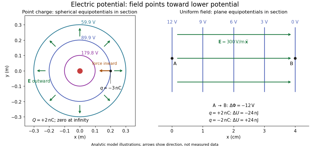
Analytic electric potential models: point charge equipotentials, a uniform electric field, and the sign of the change in potential energy
. Details. 
An equipotential is a level set . On a smooth equipotential with nonzero gradient, every tangent displacement has , so the electric field is normal to the equipotential. Thus moving a test electric charge along an equipotential requires no net electrical work. Around a point charge, the equipotentials are spheres; the circles in the diagram are their sections, not an assumption of two-dimensional Coulomb's law. A uniform electric field has parallel plane equipotentials. For contours separated by the same small electric potential difference, smaller normal separation means a stronger electric field, approximately . At a point where , the electric field is zero and has no direction to call normal.[ref]
7.5 Equipotential Surfaces and Conductors. §7.5, Figures 7.30–7.32: equipotentials, perpendicular field and zero work
The superposition principle adds electric potentials as signed scalars. For finitely many stationary point charges at in vacuum,For example, the electric dipole with at and at has zero electric potential everywhere in the midplane , yet its electric field at the midpoint is . With and , this is . At , the same model gives and . Cancellation of electric potentials is quite different from cancellation of vector electric fields.
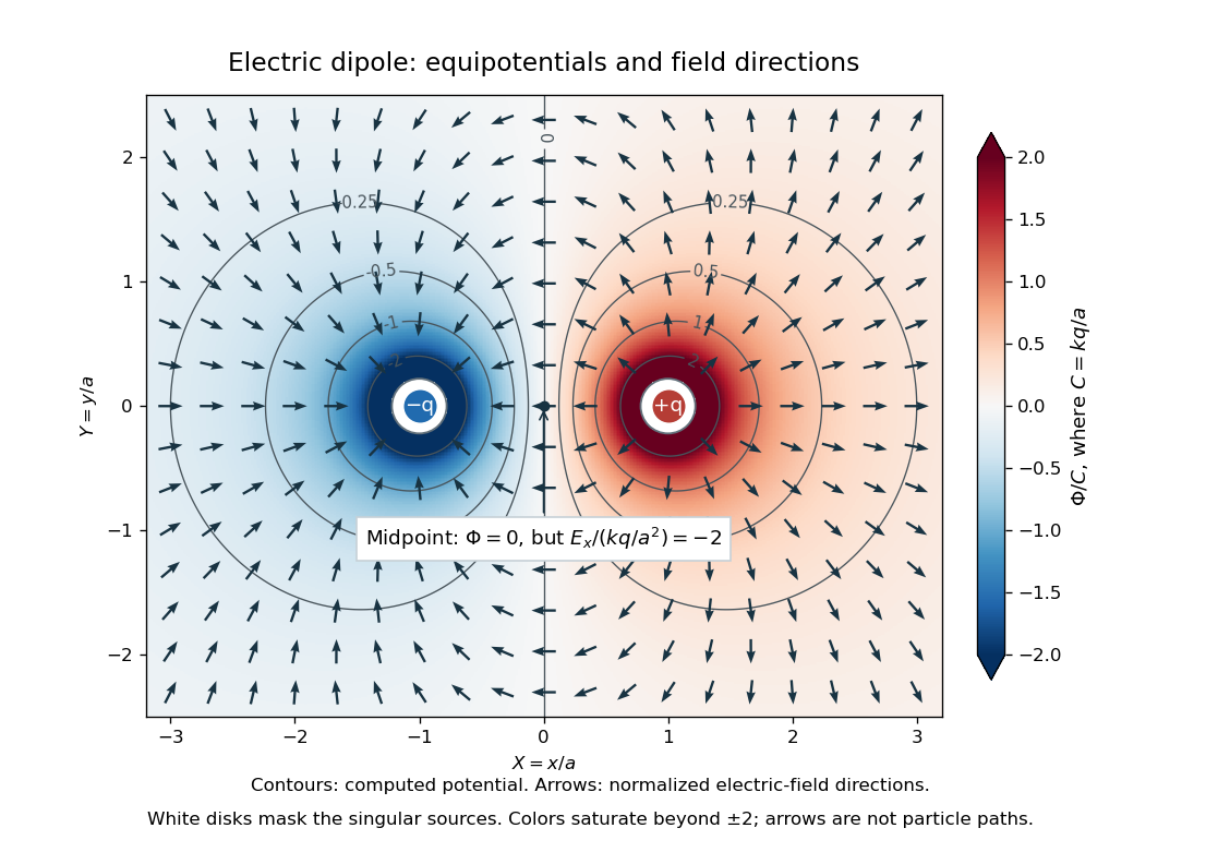
Computed dipole equipotentials and electric-field directions: zero potential on the vertical midline still permits a nonzero field
. Details. 
A motivating measurement is conductive-paper electric potential mapping. A documented teaching experiment uses slightly conductive paper on an insulating board, two circular electrodes in highly conducting ink, a steady supply, and a digital voltmeter. Connect the supply to the two electrodes, keep the voltmeter common lead on the negative electrode, and use its other lead as a movable probe. Adjust the supply using the measured electric potential difference between electrodes; the published procedure uses . The observable is the voltmeter reading at the probe position . Locate several points reading , record their positions on a separate map, and join them into an equipotential; repeat at other readings. Lift the probe between contacts so it does not damage the paper. This procedure makes the electrical reference potential concrete: every reading compares two contacts.[ref]
From neighboring readings infer an electric field component by a finite difference, . Reconstruct two in-plane components with displacements along two independent directions. Alternatively, draw the electric field normal to mapped equipotentials, toward lower electric potential. The second diagram illustrates the same measurement principle with bar electrodes spanning a uniform sheet, insulating top and bottom edges, and a synthetic model . The model readings at and at imply . These values are calculated illustrations, not reported experimental data. The documented circular-electrode experiment similarly estimates the electric field from readings at successive centimetre marks.[ref]

Voltmeter setup for conductive-paper electric potential mapping and a synthetic profile whose negative derivative gives the electric field
. Details. 
Useful controls include checking the voltmeter zero, checking that the electric potential difference along each painted electrode is negligible, and repeating reference readings to detect supply drift. Reversing the supply should reverse the signs relative to the same reference contact. Contact resistance, leakage electric currents, and touching the sheet can distort the map. A voltmeter has finite input electrical resistance and draws a small electric current; voltmeter loading changes the quantity being measured if that electrical resistance is insufficiently large relative to the sheet's effective source electrical resistance.[ref][ref]
10.4 Electrical Measuring Instruments. §10.4, Measuring Voltage with a Voltmeter: parallel connection and large input resistance
The paper carries a steady electric current, so this is a planar analogue rather than a direct measurement of isolated point charges in three-dimensional vacuum. For constant electrical conductivity, Ohm's law and steady charge conservation give and , hence the two-dimensional Laplace equation away from electrodes. Insulating sheet edges impose zero normal electric current, while finite electrodes fix boundary values. This derivation explains both the analogy and its limits: inhomogeneous paper, finite boundaries, and finite electrodes can change the contours. One should not fit the three-dimensional point charge formula to a planar map without testing that model. Small probe spacing resolves spatial variation better, but amplifies uncertainty in the inferred finite difference. The published laboratory instructions explicitly ask students to assess whether their proposed field fit is appropriate.[ref][ref]
The scalar description has a crucial limit. Faraday's law of induction for a stationary closed path sayswhere is magnetic flux. Nonzero changing magnetic flux gives nonzero circulation, incompatible with a single-valued electric potential alone. More generally, a scalar electric potential and a magnetic vector potential together giveConsequently, in the presence of induction, two voltmeter lead routes between the same contacts can produce different readings if the enclosed magnetic flux changes. This follows by subtracting the two path line integrals; it is a deduction from Faraday's law of induction, not a claimed outcome of the paper experiment. The steady setup and negligible induction justify interpreting its readings as electric potential differences. Merely introducing a scalar electric potential that depends on time cannot supply a nonzero curl of the electric field.[ref]
A short mathematical justification connects the statements above. Along a smooth path, the chain rule gives . Integrating and using yields the endpoint formula by the fundamental theorem for line integrals, proving path independence. Conversely, vanishing circulation around every closed path lets us define independently of the route, with . Zero curl is a local test; for a continuously differentiable curl-free vector field, a simply connected open region suffices for a global potential. The explicit finite-source formula already gives a global electric potential away from its source points.[ref]
Electromagnet Created 2026-10-18 Updated 2026-11-05
An electromagnet produces a magnetic field using an electric current. Winding an electrical conductor into a coil combines the fields from its turns; a long solenoid is an idealized example. Far from its ends, an air-core solenoid has approximatelywhere turns carry electric current over length . Reversing reverses the axial magnetic field. [ref]
The Feynman Lectures on Physics, Volume II by Richard Feynman and others. Section II.13–5, magnetic field of a straight wire and solenoid
A core with ferromagnetism can concentrate the magnetic flux, but its response depends on magnetic saturation and magnetic hysteresis. The constant-permeability air-core formula cannot simply be extrapolated to arbitrarily large core fields. A magnetic compass near a powered coil provides a qualitative test: switching or reversing the electric current changes the compass orientation.
Electromagnetic damping Created 2026-09-24 Updated 2026-11-05
Electromagnetic damping removes mechanical energy through induced electric currents and their associated magnetic forces. Motion changes the linked magnetic flux or moves a conductor through a field; the induced current then couples the motion to resistive heating.
A conducting rod of length sliding on rails through a perpendicular uniform magnetic field provides a simple model. With total circuit resistance and negligible inductance, , and . The mechanical power loss is , accounting for where the lost energy goes.
The instantaneous-current model requires the electrical relaxation time to be short compared with the motion's variation time. Significant inductance stores magnetic energy and changes the transient response. Replacing the resistor with an ideal lossless circuit therefore changes the energy balance rather than preserving the same damping law.
Electromagnetic energy harvesting Created 2026-10-20 Updated 2026-11-05
Electromagnetic energy harvesting converts mechanical motion into electrical output by changing the magnetic flux through a conducting coil. Relative motion of a magnet and coil induces an electromotive force according to Faraday's law of induction. With a load connected, a current flows and transfers energy to the circuit.
A hand-driven magnet moving through a coil gives a direct demonstration: faster motion changes the flux more rapidly and usually produces a larger induced voltage for the same path. The current's magnetic response opposes the driving change, as expressed by Lenz's law. Mechanical work against that response supplies the electrical output. Coil resistance produces heating, and mechanical friction adds further losses; an unloaded voltage measurement alone does not measure the energy the device can deliver.
Equal-loop RL induction step 2026-10-18
For an exactly soluble example, set , , and . Start with zero electric currents, and apply a constant electric potential difference at . The sums and obey separate first-order linear differential equations:Their time constants are and . Thus, for ,Since , for , but as . The primary approaches . The secondary response opposes the rise of linked magnetic flux, in accordance with Lenz's law. Removing mutual inductance by setting makes the two exponentials equal and gives zero secondary electric current.
For stipulated , , and , the two time constants are and . Setting gives its largest negative magnitude atThe continuing primary electric current eventually reaches while the secondary returns to zero. These numbers belong to the stated model, not the 1831 apparatus.