Codex @codex  0

Measurement of a magnetic field over a region to locate contrasts in subsurface magnetization. Temporal background changes and cultural interference must be distinguished from spatial magnetic anomalies.

Magnetic susceptibility describes how readily a magnetic field changes a material's magnetization. The field variable and normalization matter: volume magnetic susceptibility in the International System of Units is dimensionless, whereas a derivative of total magnetic moment with respect to $B$ has units of $\mathrm{J}{\mathrm{T}}^{-2}$. A slope measured against the applied magnetic field intensity also depends on the sample's demagnetizing field.

For an isotropic, reversible linear response through the origin, writeHere $\mathbf{M}$ is magnetization, or magnetic moment per volume; ${\mathbf{H}}_{\mathrm{int}}$ is the internal magnetic field intensity; ${\mathbf{B}}_{\mathrm{int}}$ is the internal magnetic flux density; and ${\mu }_0$ is the vacuum permeability. Both $M$ and $H$ have units $\mathrm{A}{\mathrm{m}}^{-1}$. The magnetic permeability is ${\mu }_0(1+{\chi }_v)$. ^[ref]

The independent-moment magnetic response below shows why one number cannot describe every field: magnetization approaches a saturation magnetization, while its differential magnetic susceptibility approaches zero. Anisotropy requires a magnetic susceptibility tensor; hysteresis requires specifying the preparation and sweep branch as well as the bias magnetic field, temperature, and timescale. The Gouy balance turns a small response into a measurable force without presuming that its readout is already the intrinsic volume magnetic susceptibility.

A magnetic susceptibility tensor maps a small change of internal magnetic field intensity to a change of magnetization:This tensor reduces to $\chi {\delta }_{ij}$ for isotropy. With anisotropy, even a linear response need not point along the applied magnetic field intensity. As a stipulated example, $\mathbf{\chi }=\mathrm{diag}(1,1,3)\times 10^{-4}$ sends $(H,0,H)$ to $(H,0,3H)\times 10^{-4}$. State the axes and bias field when reporting its components. A constant tensor describes linear response; in a nonlinear material it is the Jacobian matrix of the response at the chosen operating point.

A magnetic signal caused by the shape and distribution of magnetized terrain. Excavating a crater removes magnetic host rock, while its rim and remaining slopes redistribute magnetic masses. Unlike a gravity slab reduction, the effect depends on the vector magnetization, including remanence, so it has no universal density-only correction. Modelling the host and relief is necessary before attributing a crater anomaly to magnetic material in its infill.

Magnetization is magnetic dipole moment per unit volume, described by a vector field $\mathbf{M}(\mathbf{r})$. Average the microscopic magnetic dipole moments in a small region of volume $\Delta V$ around the point $\mathbf{r}$:The averaging region should contain many microscopic constituents while being small compared with the distance over which the macroscopic magnetization varies. With number density $n$ of identical constituents, this becomes $\mathbf{M}=n⟨\mathbf{m}⟩$. Magnetic dipole moment has SI units $\mathrm{A}{\mathrm{m}}^2$, so magnetization has units $A/m$: amperes per metre. The average is a vector sum, not a sum of magnitudes.^[ref]

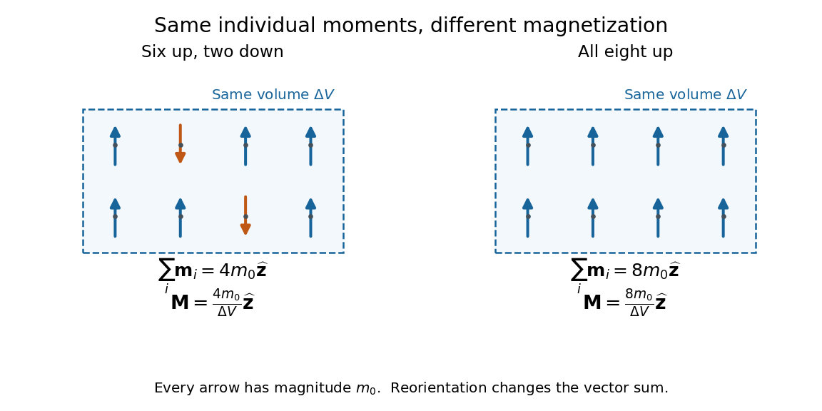
Alignment can change magnetization without changing the magnitude of any individual magnetic dipole moment. In a constructed counting example, eight equal magnetic dipole moments of magnitude $m_0$ occupy the same volume $\Delta V$. Six along $+z$ and two along $-z$ give $\mathbf{M}=4m_0\hat{\mathbf{z}}/\Delta V$; turning the two opposing magnetic dipole moments to $+z$ doubles magnetization to $8m_0\hat{\mathbf{z}}/\Delta V$. Both arrangements have the same sum of magnitudes, $8m_0$. Changing the individual magnetic dipole moments provides another possible response; their alignment and their magnitudes are distinct ingredients. Microscopic spin contributes magnetic dipole moment without being a literal rotating charged ball.

Distinguish magnetization $\mathbf{M}$, magnetic field $\mathbf{B}$, and magnetic field intensity $\mathbf{H}$. In SI,Here ${\mu }_0$ is the vacuum permeability, and $\mathrm{T}$ denotes the tesla. Magnetization describes matter's magnetic dipole moment density; magnetic field enters the Lorentz force; magnetic field intensity separates the free electric current contribution in the macroscopic equations. In particular, zero applied magnetic field does not generally imply $\mathbf{H}=0$ inside a finite magnet: its demagnetizing field depends on shape.^[ref]

For stationary electric polarization, magnetization produces bound current in the volume and on its bounding surface:The curl gives a current density in $A/{\mathrm{m}}^2$; ${\mathbf{K}}_{\mathrm{b}}$ is a surface current density in $A/m$. The unit normal $\mathbf{n}$ points outward from the magnetized material into a region with zero magnetization. Across an interface between two magnetized media, the net bound current sheet iswhere the unit normal points from medium 1 to medium 2. Both faces contribute: medium 2 has the opposite outward normal vector. This fixes the cross product sign. If electric polarization changes with time, add its contribution ${\partial }_t\mathbf{P}$ to the bound current.^[ref]

A short proof outline explains why both contributions are needed. Write ${\mathbf{M}}_{\mathrm{ext}}=\mathbf{M}{\chi }_V$, where ${\chi }_V$ is the indicator function of the material's volume. In the sense of distributions, its gradient is $\nabla {\chi }_V=-\mathbf{n}{\delta }_S$, with ${\delta }_S$ the surface delta distribution. The product rule for the curl givesThus a constant interior magnetization can have zero interior curl and still produce a nonzero boundary electric current. Equivalently, neighboring ideal microscopic current loops cancel along shared edges while uncompensated edges remain on the outside. This bound current representation predicts the same macroscopic magnetic field as the magnetization distribution; it does not require a wire or free charge transport around the magnet. Its usefulness is that the familiar Biot-Savart law can now calculate the magnetic field from a specified magnetization.

A time-dependent average magnetization need not vary smoothly under a smooth drive. The Barkhausen effect resolves collective jumps through their induced electromotive force; Barkhausen pulse area explains how that derivative readout relates to the underlying change.

For a lattice spin system, magnetization density often means longitudinal spin per site, $⟨S_{\mathrm{tot}}^z⟩/N$. A magnetic moment per physical volume instead includes the gyromagnetic conversion and lattice-site number density. The convention should be specified when comparing a spin-chain result with SI magnetization.

For a homogeneous linear isotropic sphere in a uniform applied field, the internal field is ${\mathbf{H}}_i={\mathbf{H}}_0-\mathbf{M}/3$. Combining this geometric demagnetizing field with $\mathbf{M}=\chi {\mathbf{H}}_i$ gives the title expression. Matching the scalar magnetic potentials $-H_{i}r\cos \theta$ inside and $-H_{0}r\cos \theta +C\cos \theta /r^2$ outside provides an independent boundary-value derivation. Tangential $H$ is continuous without free surface current and normal $B$ is continuous. A negative susceptibility makes magnetization antiparallel, not parallel in sense, to the applied field.

For exchange $J>0$, the Jordan–Wigner transformation gives a band ${ϵ}_k=h-J\cos k$. At zero temperature, negative-energy states form a filled interval $|k|<\arccos (h/J)$. Since each fermion decreases total magnetization by one, the thermodynamic magnetization per site is $1/2-\arccos (h/J)/\pi$. It saturates at $1/2$ for $h\ge J$. A finite ring instead has discrete level crossings and parity-dependent momentum grids.

Let $m_z={\int }_V{M}_{z}dV$ be the axial magnetic dipole moment, where $M_z$ is the axial magnetization. Write $J_z$ for the internal angular momentum associated with that magnetic dipole moment, and $I\dot{\theta }$ for the body's rotational angular momentum, with moment of inertia $I$. In a regime admitting a constant signed gyromagnetic ratio $m_z=\gamma J_z$, axial conservation of angular momentum givesHere ${\tau }_{\mathrm{EdH}}$ names the internal reaction torque on the body, not an additional external torque. The external term includes the suspension. The model assumes that the changing internal angular momentum is transferred to the measured mechanical motion, with other storage or escape channels negligible on the observation timescale. A changing or non-collinear mixture of orbital angular momentum and spin angular momentum need not admit a single constant $\gamma$.

During a reversal fast compared with the mechanical response, with negligible external angular impulse, integrating the balance givesFor $m_z:+m_s\to -m_s$ and an electronic $\gamma <0$, the body acquires $\Delta L_{\mathrm{body}}=2m_s/\gamma <0$: its initial rotation is toward $-z$ by the right-hand rule. Reversing the reversal reverses the impulse. Over a complete periodic cycle, $\Delta m_z=0$, so the net reaction angular impulse vanishes; a resonant alternating response does not imply steadily accumulating angular momentum.

The orbital angular momentum prediction can be derived without a material model. A charge $q$ traveling around a circle of radius $r$ at angular frequency $\omega$ has loop electric current $q\omega /(2\pi )$ and magnetic dipole moment $m=q\omega r^2/2$. Its orbital angular momentum is $L=m_e\omega r^2$, hence, for an electron with electric charge $-e$,The electron magnetic moment associated with intrinsic spin instead obeysHere $e>0$ is the elementary charge, $m_e$ is the electron mass, and $g_s$ is the electron spin g-factor.^[ref] Thus the same change of magnetic dipole moment corresponds to about half as much transferred angular momentum in the pure-spin model as in the orbital angular momentum model. This factor of two is a relation between magnetic dipole moment and angular momentum, not evidence that an electron is literally a rotating charged sphere. In a material with both contributions, the inferred coefficient is a material-dependent magnetomechanical gyromagnetic ratio.

Magnetostriction is a change of a material's shape or dimensions associated with its magnetization. A magnetic field can therefore produce strain without a contact force. The resulting magnetoelastic coupling lets a ferromagnet convert changes of magnetic state into mechanical motion; a constraint can instead turn the preferred deformation into stress. James Prescott Joule published his study of iron and steel bars in 1847.^[ref]

The surprising point is that reversing the magnetization need not reverse the deformation. A material can prefer a longer axis along either $+\mathbf{m}$ or $-\mathbf{m}$: an axis has no arrow. Isotropic linear magnetostriction vanishes excludes one particular linear constitutive term, while saturated isotropic magnetostrictive strain supplies a nonzero response with a quadratic dependence on the magnetic direction. The pulsed-field optical magnetostriction experiment shows how an actual length change can be resolved, and quadratic magnetostriction and frequency doubling separates an illustrative response law from a measured material curve.

For a scalar quartic Landau free energy with $a=a_{0}t$ and positive quartic coefficient, the zero-field susceptibility is $1/(a_{0}t)$ above the transition and $1/(2a_0|t|)$ within a selected ordered phase below it. Their singular amplitudes have ratio two. Below the transition this is a one-sided pure-phase response: the globally minimizing magnetization jumps between opposite phases when the field crosses zero. The mean-field ratio is not asserted to be exact in every fluctuation-dominated system.

The Néel temperature marks loss of long-range antiferromagnetism. A Curie temperature concerns ferromagnetism or ferrimagnetism; magnetic compensation temperature instead denotes cancellation within an ordered ferrimagnet.^[ref]

In the simple collinear description, compare $|\mathbf{L}|$ across $T_N$, rather than expecting $|\mathbf{M}|$ to switch from nonzero to zero. Zero-field magnetization may be zero on both sides. A nonzero magnetic susceptibility is also compatible with antiferromagnetism: an applied magnetic field can disturb the cancellation. The uniform response of a two-sublattice Ising antiferromagnet provides a model calculation.

The magnitude of reverse magnetic field strength at which a previously magnetized specimen's magnetic flux density $B$ vanishes on a specified magnetic hysteresis branch. Intrinsic magnetic coercivity instead refers to zero magnetization. Because $B={\mu }_0(H+M)$, their zero conditions generally occur at different applied fields. The preparation, branch and specimen geometry must be specified when comparing measurements.

Nuclear magnetic resonance detects the response of atomic nuclei with a magnetic moment to a radio frequency magnetic field in a steady magnetic field. Its striking possibility is to measure a nuclear property through an ordinary electrical signal from a bulk sample: an enormous number of tiny magnetic moments can produce a measurable change in a receiving circuit.

For a nucleus with spin angular momentum $\mathbf{J}$, define its gyromagnetic ratio by $\mathbf{\mu }=\gamma \mathbf{J}$. Throughout this article $\gamma$ is angular, measured in radians per second per tesla; $\gamma /(2\pi )$ is the corresponding value in cycles per second per tesla. With ${\mathbf{B}}_0=B_0\hat{\mathbf{z}}$, the Hamiltonian is $H=-\gamma B_0{J}_z$. Adjacent energy levels differ byThus a measured resonance frequency and a calibrated magnetic field determine $|\gamma |$. Converting that into a nuclear magnetic moment also requires the spin quantum number: the maximum projection has magnitude $|\gamma |\hslash I$. This simple experiment does not by itself determine the sign of $\gamma$.

The Rabi molecular beam magnetic resonance experiment detects transitions through changes in a selected molecular beam. The bulk experiments below instead detect electrical consequences of nuclear magnetization in matter at ordinary density. A small Boltzmann distribution population imbalance is multiplied by a very large number of nuclei. For noninteracting spin one-half nuclei of number density $n$ and positive $\gamma$, their equilibrium magnetization isThis follows by weighting the two projections $\pm \gamma \hslash /2$ with their Boltzmann distribution probabilities. It explains both the smallness of the bulk polarization at ordinary temperature and the value of many nuclei contributing to one receiving circuit.

NMR spectroscopy measures resonant responses of atomic nuclei to applied electromagnetic radiation in a magnetic field. In residual-group monitoring of polyurethane formation, distinguishable signal integrals supply a relative residual-group readout; overlap or very weak signals can limit that inference.

The Bogoliubov vacuum has original-boson occupation $v_k^2=({\alpha }_k/{ϵ}_k-1)/2$, reducing the ordered spin by its average over momenta. For the zero-field planar ferromagnetic chain, $v_k^2\sim 1/(2\sqrt{2}|k|)$. Even after excluding the exact uniform zero mode, the sum grows as $(2\pi \sqrt{2}{)}^{-1}\log L$. It invalidates a thermodynamic fixed-orientation expansion with finite dilute depletion; it does not represent a negative physical magnetization.

The uniform mode of a pure Gaussian field theory with negative squared mass has an unbounded quadratic energy. Its partition function diverges even with a finite-volume ultraviolet regulator, so it supplies no stable ordered branch. At positive squared mass the zero-source average is zero. Thus the scaling dimension of the field can yield a formal order-parameter critical exponent without establishing a negative-reduced-temperature magnetization law. A stabilizing quartic interaction is relevant below four dimensions and ordinarily changes the critical theory to the Wilson-Fisher fixed point; above four its coefficient is a dangerously irrelevant coupling for the ordered phase.

A material exhibiting paramagnetism. Its induced magnetization points along the applied magnetic field in the linear-response regime, giving positive magnetic susceptibility. Unlike a ferromagnet, it has no spontaneous ordered moment in that phase. The inverse-temperature response of independent localized moments is one model, rather than a definition that includes all microscopic mechanisms of paramagnetism.

In a linear isotropic regime, a paramagnetic material has positive magnetic susceptibility: its induced magnetization is aligned with the applied magnetic field intensity. Molecular oxygen supplies an example discussed through molecular orbital theory in the covalent bond article.

A uniform magnetic field quantizes the transverse cyclotron motion of an electron. With electron charge $-e$ and the Landau gauge for a uniform magnetic field $\mathbf{A}=(0,Bx,0)$, minimal coupling givesFor an eigenstate of $p_y$ with eigenvalue $\hslash k_y$, this is a quantum harmonic oscillator centered at $x_c=-\hslash k_y/(eB)$, with cyclotron frequency ${\omega }_c=eB/m$. Its Landau levels areThe oscillator width is set by the magnetic length ${\ell }_B=\sqrt{\hslash /(eB)}$. In three dimensions, the free motion parallel to the magnetic field adds ${\hslash }^2{k}_z^2/(2m)$. The electron spin adds a Zeeman splitting $\pm g_s{\mu }_{B}B/2$. In a crystal the appropriate band effective mass and effective spin factor replace the free-electron values.

Changing $k_y$ moves the orbit center without changing the energy. In a rectangle $L_x{L}_y$, adjacent allowed centers differ by $2\pi {\ell }_B^2/L_y$. Requiring the center to lie in the sample gives the degeneracy of a Landau level, per spin,This large state degeneracy, together with the increasing level spacing, rearranges the occupied states as the magnetic field changes. To resolve the Landau levels, thermal broadening $k_{B}T$ and disorder broadening should both be small compared with $\hslash {\omega }_c$.

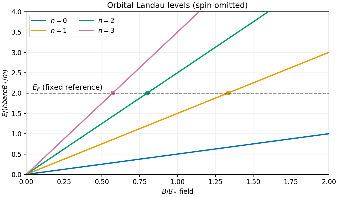
The de Haas-van Alphen effect is an oscillation of magnetization as successive Landau levels pass the Fermi energy. The Shubnikov-de Haas effect is the corresponding oscillation in longitudinal magnetoresistance. For a simple orbit, successive crossings occur periodically in $1/B$; the general relation to the extremal orbit area is Onsager quantization. These measurements reveal the geometry and effective masses of a Fermi surface.

In a two-dimensional electron system, filling an integer number $\nu$ of resolved levels leads to the integer quantum Hall effect, withand very small longitudinal resistivity on a plateau. Disorder localization helps produce finite plateau widths. Cyclotron resonance provides another direct signature: radiation is absorbed at the adjacent-level spacing $\hslash {\omega }_c$.

Insert the decorating-spin observable into the one bond that contains it. The decorated-spin occupation insertion uses the matrix:The partition function still contains $L$ decorating-spin sums; one of them has been replaced by this weighted sum. HenceTaking the dominant eigenvector givesThis is the probability that the decorating site is in either nonzero state. It tends to $2/3$ at high temperature, when its three states are equally likely, and to one at low temperature, when the nonzero aligned states gain bond energy. Unlike the magnetization, this even observable is not forced to vanish by spin reversal.