A single-walled carbon nanotube confines the electron around its circumference while allowing motion along its axis. Nanotube zone folding therefore turns the graphene bands into one-dimensional subbands. A semiconducting carbon nanotube has no allowed circumferential wave vector through a Dirac valley; a metallic tube has a band crossing at the Fermi energy in the ideal model. Each massive subband edge gives a one-dimensional van Hove singularity in the density of states, and corresponding peaks appear in the joint density of states.
For light polarized along the tube, the main electric-dipole selection rule conserves circumferential angular momentum: transitions connect matching valence and conduction subbands. These finite-energy transitions are conventionally in a semiconducting carbon nanotube and in a metallic tube. A metallic band crossing does not make its first strong interband peak have zero energy. Perpendicular polarization admits different angular-momentum channels, often much weaker because of depolarization. Excitons, dielectric screening and trigonal warping modify the simple band-edge transition energies.
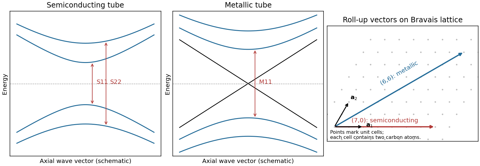
Nanotube optical transitions and two example roll-up vectors
. Original band and lattice schematics. Arrows indicate matching-subband transitions; the metallic crossing is separate from its finite-energy interband resonance. Lattice points represent graphene unit cells rather than individual atoms. Source. Details.
Experimentally, measure absorption versus photon energy; Raman spectroscopy becomes resonantly enhanced when the excitation matches an optical transition. A photoluminescence excitation spectrum of dispersed semiconducting tubes correlates excitation near with emission near after relaxation. Metallic tubes generally lack comparable bright emission because nonradiative relaxation is efficient. Combining optical energies with radial-breathing-mode Raman spectroscopy or electron diffraction assigns tube diameter and roll-up indices; a Kataura plot organizes those assignments.[ref]
Structure-assigned optical spectra of single-walled carbon nanotubes by Sergei M. Bachilo and others. Excitation-emission spectroscopy and assignments to nanotube structures
Let be equal-length primitive translation vectors of the graphene lattice, separated by . The carbon nanotube chiral vectoridentifies the two points joined when the sheet is rolled: is the circumference, not the tube axis. The right-hand panel of the preceding original diagram shows and .
The periodic boundary condition is , with an integer. Applying it at either Dirac valley gives the nanotube zone folding criterionfor a metallic tube. Thus is an armchair metallic example, whereas is a zigzag semiconducting example. Other choices with also give a semiconducting carbon nanotube.
This criterion is the ideal flat-sheet approximation. Curvature can open a small gap in nominally metallic non-armchair tubes; ideal armchair tubes remain gapless in that approximation. The property is determined by the wrapping vector, not simply by calling a tube “chiral” or by its diameter alone.
The important distinctions are changes of ring topology, missing or added atoms, and changes of local bonding:
- A Stone-Wales defect rotates one carbon-carbon bond by approximately , converting four hexagons into a --- ring arrangement without adding or removing atoms. It changes strain and electronic scattering.
- A carbon nanotube vacancy defect removes an atom. Reconstruction commonly gives a pentagon and a nine-membered ring, with an undercoordinated site; a reconstructed divacancy can give a -- arrangement. Larger vacancies make holes or broken walls.
- An adjacent pentagon-heptagon pair acts as a dislocation in the hexagonal network. It can connect regions with different wrapping indices, producing a bend or an electronic junction. Isolated nonhexagonal rings impose curvature: pentagons favor positive curvature and heptagons negative curvature.
- An interstitial defect, an adsorbed atom, or chemical functionalization can distort the network and locally change bonding toward . These defects can scatter carriers and create chemically reactive sites.
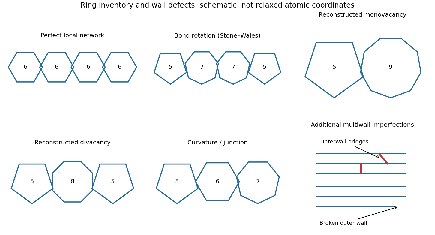

Closed end caps require nonhexagonal rings, typically six pentagons per hemispherical cap; these are part of the cap topology rather than necessarily damage. Kinks, buckling, branches and incomplete closure are larger-scale structural imperfections.
A multi-walled carbon nanotube can contain any of these defects in individual shells, plus interrupted or terminated shells, extra incomplete graphitic layers, irregular interwall spacing, and covalent interwall bridges formed by displaced atoms. Such bridges change intershell coupling and sliding. Different shells having different wrapping indices is normal and is not, by itself, a defect.
Two layers need not have the same electronic structure everywhere. Different rotational alignments create domains of twisted bilayer graphene; AB-stacked regions instead have the usual coupled low-energy bilayer bands. In a twisted domain, displaced Dirac cones hybridize where they meet, producing avoided crossings and saddle points in the two-dimensional dispersion relation. The resulting Van Hove singularities enhance optical transitions at energies that depend on the twist angle. Different domains therefore absorb different parts of the visible spectrum and can show different colours despite having the same layer count.[ref]
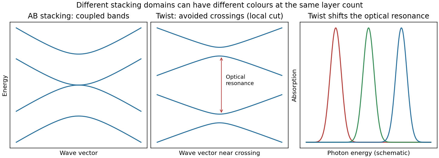
Bilayer stacking changes the bands and optical absorption
. Original illustrative bands: AB-stacked bands, a local cut through avoided crossings in a twisted domain, and schematic angle-dependent absorption peaks. The middle panel is a local cut, not the entire two-dimensional band structure. Source. Details.
On a silicon/silicon-dioxide substrate, reflected beams from the film stack also interfere. The wavelength-dependent optical response of the bilayer graphene changes this reflected contrast, making the domain differences visible. The observation is consistent with stacking domains; colour alone does not uniquely prove a twist angle. Variations in oxide thickness, trapped contamination, folds or local doping can also change contrast and should be checked independently, for example by Raman spectroscopy.
The gas impingement flux onto a surface follows from the normal component of the Maxwell-Boltzmann distribution:Here and , givingAssume a conventional monolayer density and unit sticking coefficient. The incident-monolayer time isThus a few milliseconds is the usual contamination-time estimate at this pressure.
The assumed molecular footprint matters: neither nor the sticking coefficient is specified. More generally if the sticking probability is and desorption is negligible. Water can desorb rapidly from clean graphene at room temperature, so the incident-monolayer estimate does not establish that a stable, complete water layer actually forms in that time. Residues and defects can increase local adsorption.
An atomic layer deposition recipe depends on the surface chemistry during the first cycles. A silicon wafer normally carries native oxide with reactive hydroxyl groups. A pristine graphene basal plane has no comparable dense population of dangling bonds or hydroxyl groups, so precursor adsorption and initial nucleation are much less uniform.
Consequently the nominal number of cycles calibrated to give on silicon can instead give isolated alumina islands, preferential decoration of edges, grain boundaries and defects, and uncovered graphene between islands. Adsorbed transfer residues may provide additional, irregular nucleation sites. Once alumina has nucleated, later cycles grow on the alumina normally; the problem is delayed, spatially uneven nucleation. The resulting local island height can exceed the film's area-averaged equivalent thickness.[ref]
Atomic layer deposition of metal oxides on pristine and functionalized graphene by Xinran Wang and others. Pristine graphene nucleation at edges and defects, and uniform growth after noncovalent functionalization
Two suitable improvements are:
- Introduce a dense, controlled nucleation layer, for example a noncovalently adsorbed functional layer carrying reactive groups or a very thin oxidized metal seed. This supplies precursor-binding sites while limiting damage to the conducting carbon network.
- Optimize initial exposure rather than reuse the silicon recipe unchanged: use longer precursor residence/soak times and suitably reduced initial temperature to increase adsorption and nucleation, then continue normal cycles after closure. Direct sub- continuous growth with extended residence times has been demonstrated.[ref]Parameter space of atomic layer deposition of ultrathin oxides on graphene by Adrianus I. Aria and others. Pulse/residence-time control of initial nucleation and continuous ultrathin films
Ozone or a mild plasma is another possible activation route, but it must be controlled because creating covalent defects can degrade the electrical properties that motivate using graphene.
Take a two-dimensional conducting sheet in the plane with magnetic flux density and electric current density along . Moving carriers feel the transverse Lorentz force . They accumulate at opposite edges, producing a transverse electric field until its force balances the magnetic deflection:For the transverse-voltage convention , this gives andThe Hall effect therefore measures carrier sign as well as density in the single-carrier approximation: electrons give the opposite transverse-voltage sign from positive carriers. Some tensor conventions call rather than ; the physical sign is fixed by the stated lead and field directions.
The Hall voltage is the integral of this transverse electric field across the sample width. In a three-dimensional slab of thickness , its magnitude is ; for a sheet, use the sheet number density and omit .
In the classical single-carrier model,for a two-dimensional sheet. The curve is a straight line through the origin, with its sign determined by the carrier charge and the voltage convention. The sheet Hall coefficient has units , consistent with the numerical slope used later.
The classical transverse response is not quantized. With carrier density and scattering parameters fixed, reversing reverses the transverse signal. Several carrier populations can produce a nonlinear classical curve, so straight-line behaviour here uses the stated single-population approximation rather than being a property of every conductor.
The integer quantum Hall effect requires a conducting two-dimensional electron gas with well-resolved Landau levels. In the simple parabolic-band model their orbital spacing isLow temperature and sufficiently low disorder broadening are needed so that and the relevant level width are small compared with this spacing. A high-mobility sample with is therefore useful.
Some disorder has a constructive role: localized states between extended Landau-level states allow the Fermi energy to move through a range of carrier populations while the transport response stays on a plateau. The longitudinal response is then very small and the transverse response is quantized. Whether odd or only even integer plateaux are resolved also depends on whether spin splitting is resolved.
On an integer plateau the sheet transverse resistivity has magnitudewhere the integer counts occupied resolved quantum Hall edge states. Increasing at fixed sheet density reduces the Landau filling factor . The observed trace is therefore a staircase toward larger , with transitions between plateaux rather than the classical straight line. In the plateau regions ; dissipative peaks occur at transitions.
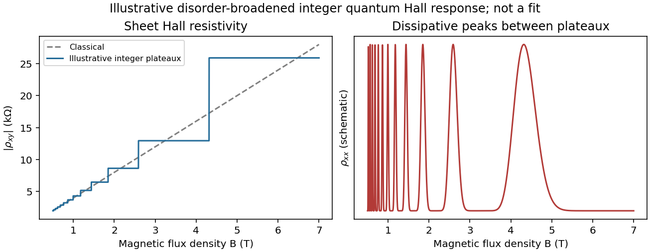
Classical Hall line and illustrative integer quantum Hall plateaux
. Original schematic responses, with the classical slope fixed by the later calculation. Plateau widths and dissipative peak shapes are illustrative rather than fitted to an experimental trace. Source. Details.
It is not correct to demand an exactly integer value of everywhere along a finite-width plateau. Localization accommodates changes in total population without changing the number of extended current-carrying channels. If spin remains unresolved, the usual spin-degenerate sequence contains even integers rather than every integer.
Using the magnitude of the classical slope,The Landau filling factor at isUnder the convention that the “last Landau level” means the last resolved spin branch, its degeneracy per area is . Setting givesAbove this threshold all carriers fit into that lowest resolved branch, which is partially filled when .
There is a spin convention to state explicitly: if “Landau level” instead means one orbital level with unresolved twofold spin degeneracy, its capacity is , and all carriers first fit into orbital index at , where . The slope alone determines and , but does not specify the spin splitting.
The giant magnetoresistance mechanism is spin-dependent conduction through the two ferromagnets. Exchange splitting gives majority and minority bands different density of states values at the Fermi energy. Scattering into those bands, together with interface scattering, produces different resistances for the two spin channels. The relevant quantity is the spin-dependent transport/scattering rate, not simply a count of all available states.
For parallel layer magnetizations, one global spin channel encounters relatively weak scattering in both Co and NiFe, providing a low-resistance path. For antiparallel magnetizations, each global spin channel encounters one more strongly scattering ferromagnet, so both paths are comparatively resistive. The channels conduct in parallel while each crosses the layers in series. This is current-perpendicular-to-plane magnetoresistance, because the current crosses the interfaces.[ref]
Nobel Lecture: Origin, development, and future of spintronics by Albert Fert. Spin-dependent conduction and the distinction between CPP and CIP transport
In the simplest two-current resistor model, with equal magnetic layers having channel resistances and spacer resistance per channel,Real Co/NiFe layers need not have equal parameters, but the same-sign spin asymmetries normally give . Their different magnetic coercivities allow the two configurations to be selected separately.
Assume NiFe is the softer layer, with , and that interlayer coupling is weak enough to permit separate reversal. Starting at large negative , both magnetizations point in the same direction and . During an increasing-field sweep:
- At , NiFe reverses while Co does not: the state is antiparallel and the resistance rises to .
- At , Co also reverses: the state becomes parallel and the resistance returns to .
On decreasing from positive saturation, the high-resistance window instead lies between and . Thus the two sweep directions give displaced rectangular high-resistance windows, not a single reversible resistance peak centered on zero.
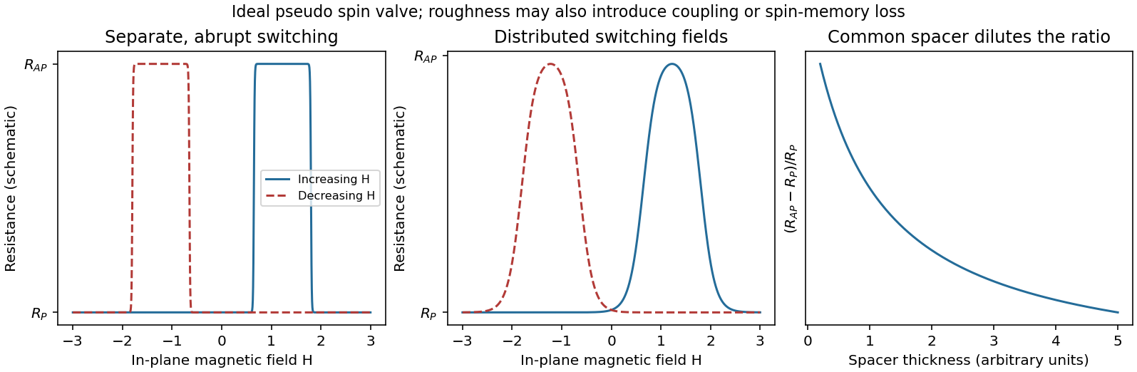
Pseudo spin-valve resistance loops, distributed switching and spacer dilution
. Original illustrative curves. Separate coercive fields create an antiparallel window on each sweep. The middle panel isolates switching-field broadening; its retained peak height is not a claim that real roughness leaves the GMR amplitude unchanged. Source. Details.
If Co were the softer layer, the sequence of layer labels would be exchanged. A continuous spacer and sufficiently weak coupling are additional assumptions: negligible surface roughness alone does not guarantee independent switching at every Cu thickness.
Specify the magnetoresistance ratio as . Increasing a continuous Cu spacer adds spin-independent series resistance. Even when remains below the spin diffusion length, this dilutes the ratio; spin information need not be destroyed to reduce the percentage signal. In the illustrative two-current resistor model,which decreases as increases. The absolute difference also decreases in this model. At a fixed bias current, the measured voltage contrast is .
For comparable to or greater than the spin diffusion length, additional spin relaxation further suppresses the contrast. At the other extreme an ultrathin or discontinuous Cu layer can introduce direct magnetic coupling or pinholes, preventing a fully antiparallel state. Thickness-dependent interlayer coupling can therefore make the very-thin-spacer trend nonmonotonic; a universal exponential law does not follow from the supplied assumptions.
Roughness can produce a distribution of local switching fields and nonuniform reversal. The abrupt edges in the ideal pseudo spin valve loops then become rounded or sloping, the antiparallel plateau becomes less flat, and overlapping layer-reversal distributions can narrow or partly eliminate the clear high-resistance window. The middle panel of the original diagram illustrates only this broadening mechanism.
Correlated roughness on the two interfaces can also introduce orange-peel coupling, a magnetostatic coupling that favors parallel alignment. Such coupling shifts switching fields and can suppress independent reversal. Sufficiently severe roughness or pinholes can have a similar qualitative effect by directly coupling the ferromagnets.
Changes in amplitude require care. Some spin-dependent interface scattering contributes to giant magnetoresistance, so a small increase in roughness is not guaranteed to lower the signal monotonically. Intermixing, spin-flip scattering and an incompletely antiparallel state generally reduce useful contrast. The detailed width, displacement and height of therefore depend on how the interfaces become rough, rather than on a single roughness number.
Two practical approaches retaining Co and NiFe are:
- Improve the spin-selective interfaces: control deposition and intermixing, avoid oxidation or magnetic dead layers, and reduce pinholes and spin-flip defects. The aim is large majority/minority transport asymmetry with low spin-memory loss, rather than merely the smallest total resistance.
- Optimize the Cu thickness and electrical stack: use the thinnest continuous spacer that still allows independent layer reversal and remains well below its spin diffusion length; reduce extraneous contact or lead resistance. This preserves a full antiparallel state and limits spin-independent dilution of the measured magnetoresistance ratio.
Increasing magnetic-layer thickness toward the useful spin-dependent-scattering scale can be another optimization, but growth beyond the relevant spin diffusion scale eventually gives diminishing returns. Merely increasing the bias current increases the readout voltage and possible heating; it does not, by itself, increase the intrinsic giant magnetoresistance ratio.
The Flory interaction parameter measures the free-energy penalty of unlike block contacts relative to like contacts, in units of . The degree of polymerization counts the reference segments per chain, using the segment-volume convention associated with . Their product, the block copolymer segregation strength , compares the tendency to avoid unlike contacts with the entropy cost of organizing and stretching connected chains.
At small , the diblock copolymer is disordered. Increasing can cause microphase separation: the blocks form distinct domains, but their covalent connection prevents complete macroscopic separation. Domain interfaces cost energy while chain stretching and lost configurations cost entropy; their competition selects a finite domain scale.
A common temperature law is , so increasing temperature often decreases segregation when . This is not a universal sign law for every polymer pair. For an intact, fixed chain, does not change just because temperature or solvent concentration changes.
Adding a nonselective good solvent usually dilutes unlike-block contacts and reduces an effective segregation strength; it does not chemically shorten the chain. A selective solvent additionally changes domain swelling and solvent-block interactions. One needs a ternary-mixture description, or a clearly defined effective , rather than treating the melt's as a universal solvent-concentration function.[ref]
Polyisoprene-polystyrene diblock copolymer phase diagram near the order-disorder transition by Ashish K. Khandpur and others. Definition of the segregation and composition variables and experimental phase behaviour
For the dry diblock copolymer, the block volume fractionis the volume assigned to the polyisoprene block divided by total polymer volume, not its mass fraction or the volume fraction of polymer in the whole solution. It controls domain curvature and topology. Similar block volumes favor alternating lamellae; a smaller minority block generally favors curved interfaces, cylinders and eventually isolated spherical domains.
The chemical block lengths are fixed. Temperature changes their volumes only through thermal expansion, so is often approximated as temperature independent; unequal expansion coefficients can produce a small change.
Solvent requires a distinction between dry composition and swollen domain composition. The dry remains fixed. If solvent volumes and partition into the two domains, an effective swollen fraction isA polystyrene-selective solvent therefore lowers , whereas a polyisoprene-selective solvent raises it. Equal proportional swelling leaves this effective ratio unchanged.
Reading the lowest point of the order-disorder boundary in the supplied experimental diagram gives approximately(about –, allowing for the graphical resolution). The ordered region just above that minimum is lamellar.
This is a reading of the supplied polyisoprene-polystyrene phase diagram. It should not be replaced by the often quoted symmetric-chain mean-field theory value : that refers to a different idealization and is not the minimum drawn here.
The starting point is in the lamellar region. Preferential swelling of polystyrene makes polyisoprene the increasingly small minority domain, so the relevant effective composition moves left from .
If segregation stayed near , following the horizontal path in the supplied diagram would give lamellae → hexagonally perforated layers → hexagonally arranged PI cylinders → PI spheres, before sufficient asymmetry reaches the disordered region. The perforated-layer interval is narrow, around – at this segregation strength; precise boundaries should not be read more accurately than the figure allows.
Solvent also changes effective segregation, so the actual trajectory need not be horizontal. If it passes closer to the order-disorder boundary, it can enter the narrow double gyroid region instead of, or after, the hexagonally perforated layer phase. Greater dilution can cause disorder before all the ordered morphologies appear. Thus a plausible alternative is lamellae → gyroid → cylinders → disorder.
The robust prediction is the change toward minority-PI curved structures, not a guarantee that every named phase occurs. A solvent partition coefficient and a concentration-dependent interaction model would be needed to locate the actual path quantitatively; applying a dry-melt diagram to a swollen material is an effective approximation.
Refraction changes the propagation direction, and hence the momentum, of transmitted light. The particle receives the opposite momentum change by conservation of momentum. For a ray carrying power , a useful force scale iswith corrections for reflected rays and their momentum fluxes. Here is the surrounding refractive index; this is a ray-force scaling rather than a complete electromagnetic stress calculation.
For fixed geometry and refractive indices, , so the force contribution is proportional to the local intensity . Refraction toward the normal on entry and away from the normal on exit must both be included: a force inferred from only the first interface can have the wrong direction.
The specified size is larger than the wavelength, so a geometrical optics treatment is appropriate despite the generic “nanoparticle” label. A dipole/Rayleigh-particle formula would use the opposite size limit.
Because the sphere lies below the optical axis, a ray passing through its upper half samples a brighter part of the Gaussian beam than a comparable ray through its lower half. For a particle with higher refractive index than its surroundings, the stronger upper ray is deflected downward overall and transfers an upward reaction to the particle. The weaker lower ray gives a smaller downward reaction. Their transverse sum is therefore upward, toward the brighter axis.
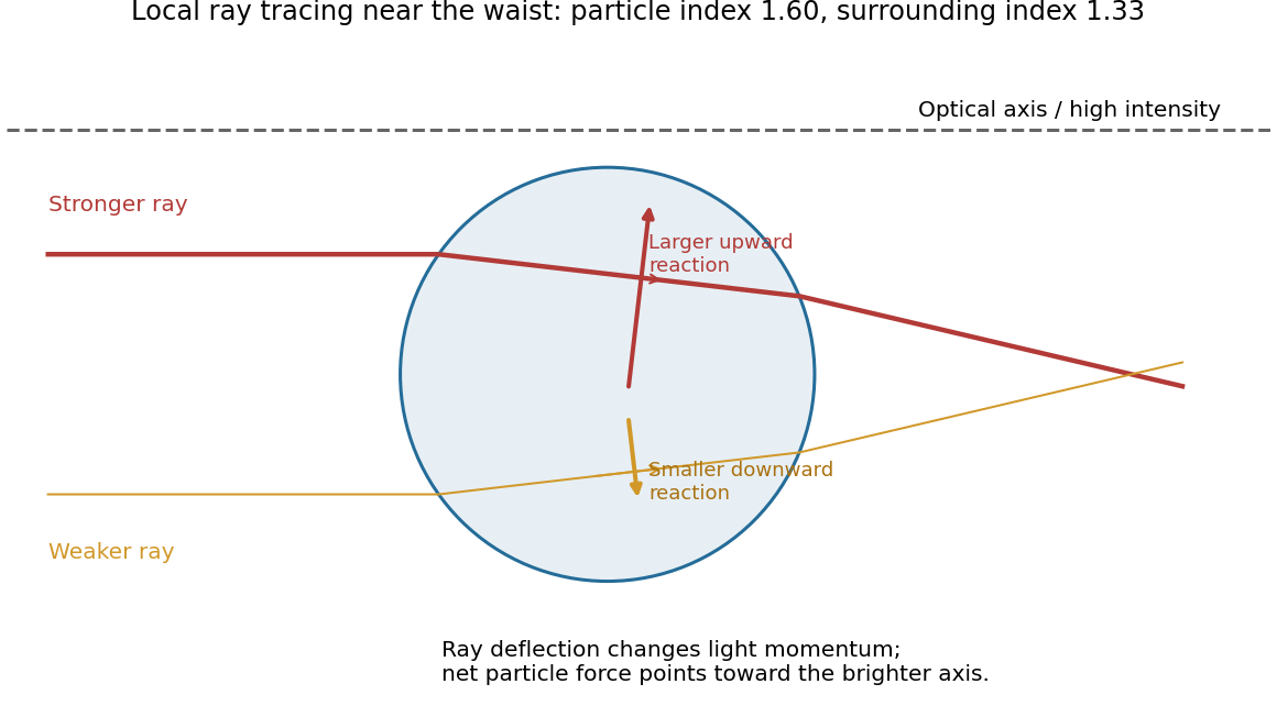
Unequal refracted rays give a transverse restoring force
. Original local ray tracing near a beam waist, with chosen refractive indices. The sphere is below the optical axis. The stronger ray contributes the larger upward reaction; the diagram isolates transverse restoration rather than reconstructing the examination figure. Source. Details.
If the displacement reverses, the force reverses, so the central position is transversely stable. Summing all the rays gives an optical gradient force toward the intensity maximum. There is also a forward optical scattering force. A tightly focused beam can have an axial restoring component that balances it, generally at a small displacement downstream of the ideal focus.[ref]
Observation of a single-beam gradient force optical trap for dielectric particles by Arthur Ashkin and others. Single-beam trapping by a sufficiently strong intensity gradient
Three-dimensional stability requires the restoring axial component to exceed the forward force over part of the trajectory. A Gaussian transverse intensity profile alone does not prove that condition; insufficient focusing can yield transverse confinement while the particle still moves downstream.
Homeotropic anchoring means that the nematic director is locally normal to the particle surface, hence radial on a sphere. Far away, the uniform nematic liquid crystal has a fixed director , with and physically equivalent.
One plausible configuration is a quadrupolar Saturn-ring defect: the director is radial near the particle, bends into far away, and has a disclination loop just outside the particle's equator, in the plane perpendicular to . A meridional section cuts the loop at two points.
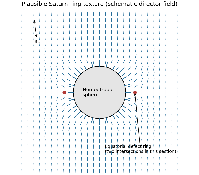

The defect compensates the topological distortion introduced by the radial surface boundary condition. A dipolar configuration with a nearby hyperbolic point defect is another possible texture. Which is stable depends on particle size, anchoring strength, elastic constants and external confinement; the boundary conditions alone do not uniquely select one.[ref]
Director field configurations around a spherical particle in a nematic liquid crystal by Holger Stark. Competing dipolar, Saturn-ring and surface-ring configurations
Absorption converts part of the incident optical power into heat. Increasing laser power can therefore raise the local temperature, potentially driving a thermotropic nematic liquid crystal through its nematic-isotropic transition. The associated loss or change of orientational order, refractive index and anchoring can alter the trapping force or destabilize the trap.
Even below that transition, thermal gradients can induce convection, thermophoretic drift and changes in viscosity or Brownian fluctuations; sufficiently strong heating can damage the particle or host. Thus increasing laser power need not simply strengthen an otherwise unchanged optical trap.
Nucleation is the formation of a sufficiently large embryo of the new metallic phase. Producing metal atoms from dissolved precursor can create supersaturation; aggregation lowers bulk free energy but initially creates costly metal-medium interface. In the simplest spherical classical nucleation theory,where is the metal-medium interfacial free energy and is the bulk driving force per volume. Clusters below the critical size tend to redissolve; larger ones can grow.
In homogeneous nucleation, the critical cluster forms in the solution without a pre-existing interface: the initial products are free particles. In heterogeneous nucleation, a substrate, vessel wall or suspended seed replaces part of that costly new interface. For a spherical cap on a planar substrate,A wetting substrate therefore lowers the barrier; this assumes the same bulk driving force and isotropic interfacial energies.
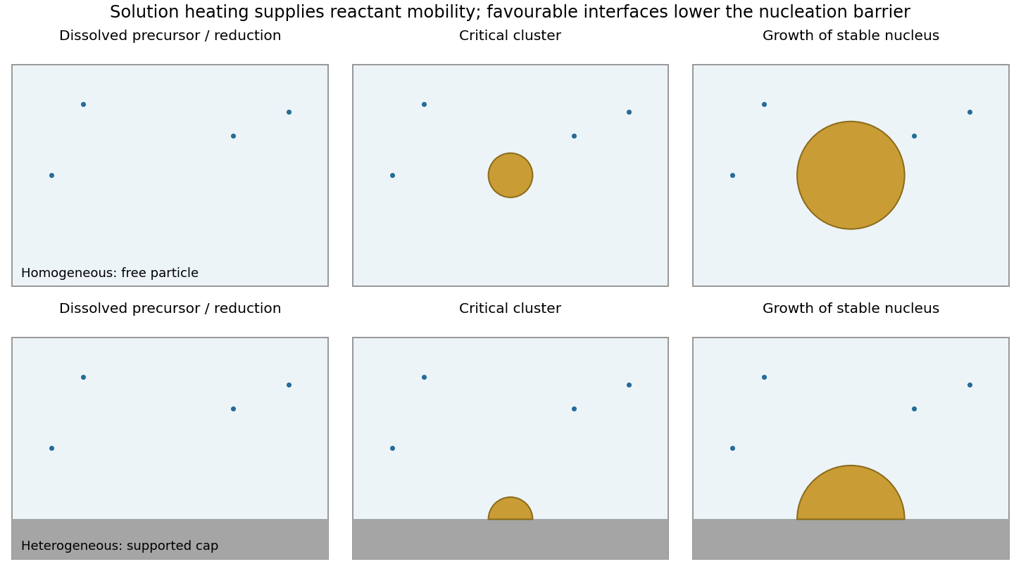

A final supported particle need not have nucleated heterogeneously: a free particle can nucleate in solution and later adsorb on the support. Conversely, a particle nucleated heterogeneously on a suspended seed can remain freely dispersed as a composite particle. Nucleation location and final support status are different classifications.
Microwave absorption heats the medium and possibly the support, changing reduction, diffusion and supersaturation. Preferential local heating can change the relative rates of the two routes. Microwave irradiation alone does not remove the thermodynamic nucleation barrier or demonstrate a special nonthermal mechanism.
- Can the precursor produce metal? Evaluate the reaction Gibbs free energy, including reduction, ligand exchange, precursor and reductant activities, solvation and byproducts. A nominal metal concentration is not the metal-atom chemical potential.
- What is the driving force for condensation? Compare the chemical potential of available metal species with that of the condensed phase. The resulting supersaturation supplies the bulk free-energy gain and competes with the surface cost of a critical nucleus.
- Where does it wet and nucleate? Let , and denote support-medium, particle-medium and support-particle interfacial free energies. For an isotropic cap, the contact angle through the particle obeys . This wetting balance determines the extent of substrate contact and the heterogeneous barrier.
- Which crystal faces survive? At fixed particle volume, minimize the sum of orientation-dependent surface and interface energies, plus any important strain or defect energy. For a free crystal, the Wulff construction gives facet distances proportional to their surface free energies. A Winterbottom construction incorporates the support interface and truncates the corresponding equilibrium shape.
Adsorbed ligands and solvent can change different facet energies by different amounts, so the relevant energies belong to the actual chemical environment. Small particles have large surface-to-volume ratios and are particularly sensitive to these terms.
This sequence identifies thermodynamic factors rather than guaranteeing that an equilibrium shape is reached. Facet-specific attachment rates, precursor delivery and limited annealing can preserve a kinetically selected shape even when another shape has lower free energy.
Write the reaction using the species actually supplied by solution. For either halide, a bulk contribution per converted formula unit isThe stated room-temperature feasibility means that the overall reaction free energy is negative under those conditions; it does not say that each microscopic step is downhill. Equal nominal concentrations also do not make iodide and bromide activities or solvation free energies identical.
At the nanoscale the balance additionally contains changing interfaces:Here is the number of converted formula units, and includes solvent-facing surfaces and contact with the titanium-dioxide support. Surface terms scale approximately as size squared whereas bulk terms scale as size cubed. Particle size, wetting, expansion during conversion and new grain interfaces can therefore shift both the conversion driving force and the nucleation barrier.
Microscopically, conversion requires desolvation, uptake of the organic cation and halide, redistribution through the precursor, and reorganization of the lead-halide framework. A study using these conversion conditions found energetically costly dispersed-ion intercalation for both compounds, with a much larger calculated penalty for MABr in PbBr than for MAI in PbI. The iodide's layered framework accommodates the cation more favorably; the bromide's undulated framework gives poorer coordination and greater local distortion. Stabilization on forming intermediate compounds and the final perovskite can nevertheless make the complete reaction favorable. The calculations are approximate energetic comparisons, not measured finite-temperature activation free energies.[ref]
Kinetics and energetics of metal halide perovskite conversion reactions at the nanoscale by Neha Arora and others. Fig. 4 and accompanying discussion: solvation reference, intercalation and conversion intermediates
Thus both reactions can be spontaneous yet proceed at very different rates: the same study observed faster MAPbI formation. One must distinguish net reaction free energy from intermediate penalties and diffusion barriers. Spontaneity alone supplies no quantitative ranking of the complete iodide and bromide reaction free energies.
In catalytic chemical vapor deposition, a metal nanoparticle activates a carbon-containing feedstock and supplies mobile carbon to the growing rim. Carbon can diffuse over the particle surface and, depending on the catalyst state, through its bulk. Once a curved carbon cap nucleates, continued incorporation extends the tube. Strong catalyst-support adhesion favors base growth; weaker adhesion can allow the particle to lift with the tube tip. A liquid catalyst is not universally required.
Particle size constrains tube diameter, but semiconducting character requires a particular wrapping family: . Merely making particles smaller does not select that congruence class. Routes toward predominantly semiconducting carbon nanotubes include controlling catalyst composition, exposed facets and size distribution to bias cap/rim nucleation and growth, or adjusting carbon chemical potential and growth/etching conditions so that metallic tubes are less likely to survive.
These are mechanistic strategies rather than a universal recipe. Experiments with catalyst conditioning found that high semiconducting selectivity depended sensitively on oxidizing/reducing gas conditions and came with a strong yield penalty, motivating a catalyst-deactivation model.[ref]
A phenomenological model for selective growth of semiconducting single-walled carbon nanotubes based on catalyst deactivation by Shunsuke Sakurai and others. Catalyst conditioning, gas composition and selectivity-yield tradeoff
The useful distinction is between selecting a structure at nucleation, selecting its growth rate, and selectively terminating or removing unwanted tubes. Each can enrich the semiconducting fraction, but they do not establish the same growth mechanism.
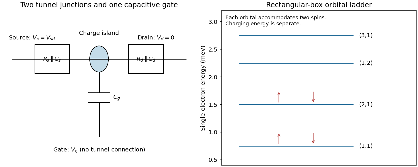
The pattern is characteristic of a single-electron transistor: a small conducting island is connected to source and drain by two tunnel junctions, and to a gate through a capacitance. Inside a Coulomb diamond, changing the island's integer charge costs more energy than the leads can supply, so sequential tunnelling is blocked. Outside it, an island electrochemical potential lies in the transport window and current can flow.
For clear Coulomb blockade, the island charging scale must exceed thermal broadening, and the tunnel junctions must be sufficiently resistive to preserve well-defined charge states:in the simplest circuit. Stray capacitances should be included in if appreciable. The gate changes electrostatic energy but should not provide a conducting leakage path. Lifetime broadening and cotunnelling should be small enough not to wash out the blocked regions.

The almost identical unconfined diamonds are consistent with a constant interaction model having negligible or unresolved changes in single-particle level spacing.
The zero-bias gate period in the first plot is . In the constant interaction model, changing the gate-induced island charge by one electron givesThe tip is at above or below zero; use this half-height, not the full vertical extent. The addition energy is , giving
To distinguish the junction capacitances, explicitly adopt the circuit convention and . The diamond with zero-bias endpoints and has its positive tip near . Its two edge slopes are therefore and .
Writing the island electrochemical potential as a charge-dependent constant minus , alignment with the drain gives slope , while alignment with the source gives . ThusThe source/drain names are exchanged if the opposite lead is biased under the voltage convention. The figure alone establishes the pair unless that wiring convention is specified. Symmetric-looking diamond heights do not imply equal junction capacitances.
Inside the rectangle the effective-mass Schrödinger equation iswith at all four walls because the confining potential is infinite outside. Separate . Each factor obeys a one-dimensional particle in a box equation. For ,so is proportional to with ; the zero and negative integers give no new physical states. The same argument applies in .
The normalized spatial states and their energies areThe product form and energy sum follow from separability. Each spatial orbital can accommodate two opposite-spin electrons under the stated spin degeneracy. These are single-particle confinement energies; the electrostatic charging contribution must still be added when interpreting transport addition energies.
The enlarged diamonds reach instead of . Subtract the unchanged charging contribution:Thus the two observed closed-orbital gaps are each approximately .
Define and , and choose the labels so . With two spins per orbital, the first two closed orbitals correspond to occupancies and . The lowest state is and the next is , soThe next orbital is , yielding the second observed gapThis ordering is self-consistent: , , and , as shown in the original level diagram.
Using givesThe axes can be interchanged. Assigning the same directly to both and would instead give a square box with degenerate and orbitals. That would require four electrons in that shell and would not give the stated second closed-orbital occupancy .
At terminal speed the downward buoyant weight balances the Stokes drag:Positive gives downward settling; a lighter particle would rise. With , , and ,about , or per day.
The very small Reynolds number makes inertial corrections to Stokes flow negligible for an isolated particle. On short particle-scale distances, Brownian motion is much faster than this systematic drift. Nevertheless the nonzero settling speed can produce concentration gradients over sufficiently long times and large sample heights; Brownian motion does not cancel gravity.
The sedimentation scale height simplifies because the same drag coefficient controls both drift and diffusion:Applying the given criterion givesEquivalently, the gravitational Péclet number on the particle-radius scale is and must be at most one.
At the limiting radius is , corresponding to diameter approximately . Viscosity cancels from this equilibrium criterion, although it affects the time to approach equilibrium.
For the radius particle in part (i), and , about particle radii. It is therefore firmly diffusion-dominated on its own size scale. This does not mean uniform concentration over an arbitrarily tall vessel: the equilibrium density still decays on the finite scale . The supplied size criterion is an approximate gravity-versus-diffusion criterion, not a universal definition of every stable colloid.
Articles were limited to the first 100 out of 105 total.
Articles by others on the same topic
There are currently no matching articles.