Original paper: Public original, physical PDF pages 261–264.
For a fixed linear circuit, self-inductance relates the magnetic flux linkage produced by its own current to that current: , with . The self-induced electromotive force is when is constant. Its unit is the henry, .
mutual inductance relates the linkage in one circuit to current in another: and . For stationary reciprocal linear media, with consistently oriented turns, and . Orientation fixes the sign. The coupled magnetic energy is , so positivity requires . Moving coils or nonlinear cores require differentiation of the full linkage rather than treating the inductance as a constant.
Use local east, north and up axes. At latitude , and eastward velocity is . The Coriolis acceleration isIts horizontal part is southward, so the lift must acquire a northward component: bank left, with the north wing lower. For the requested local Coriolis correction, let the vertical lift balance . The Coriolis bank angle for eastward flight isUse and . Including the upward Coriolis term replaces by and changes the answer by only about . This is the horizontal Coriolis compensation, not a full calculation of a curved constant-latitude flight path. The rotation rate follows Earth's sidereal period.[ref]
Earth Fact Sheet by National Aeronautics and Space Administration. Orbital parameters: sidereal rotation period 23.9345 hours
Let be heat extracted from the cold reservoir, the heat delivered to the surroundings and the supplied work. The entropy inequality for a cyclic refrigerator isEquality is the reversible Carnot refrigerator limit. Thereforeenergy conservation gives . The requested rejected heat is 75 J, while 74 J is the minimum work; both have to be distinguished. Any entropy production increases the required rejection at these fixed reservoir temperatures.
For a plane wave propagating along in vacuum, Maxwell equations give , with . HenceTaking , the period average of the squared cosine is . ThusThe fields are in phase, so the travelling-wave energy flux never reverses. The peak amplitude convention is essential; using a root-mean-square electric field would remove the factor .
Use a circular Kepler orbit to eliminate the terrestrial gravitational parameter: is constant for both satellites. The reference orbital radius is , measured from Earth's centre. A geostationary orbit is circular, equatorial and prograde, with the sidereal rotation period, approximately . ThusIts altitude is about above the stated surface. The approximate low-orbit input sets the accuracy; replacing it by a modern measured gravitational parameter would answer a different numerical estimate. A -hour approximation changes the radius by less than . Matching the period alone would not make an inclined or eccentric orbit stationary above one point.
displacement current completes Ampère's law:In vacuum . Taking the divergence and using gives , exactly the continuity equation. Without the added term a time-dependent charge distribution would contradict the curl equation.
A charging parallel-plate capacitor illustrates the physics. For plate area , , so the gap displacement current is , equal to the conduction current in its leads. An Ampère contour therefore gives the same magnetic circulation whether its spanning surface crosses the wire or the gap. No electrons have to cross an ideal vacuum gap. In matter, includes the polarization response as well as the vacuum term. Combined with Faraday induction, the displacement term permits source-free electromagnetic waves.
A thin pillbox applied to and a thin rectangular contour applied to the magnetostatic Ampère law giveThe normal points from medium1 to medium2, and is a free sheet current. Without such a current, tangential is continuous; normal is continuous independently. The remaining components need not be continuous because contains the magnetization.
For linear isotropic media with no free sheet current, and . If measures a field-line angle to the normal, . This magnetic field-line refraction follows from the two different component conditions, not from continuity of the complete vector field. Bound surface currents are already represented in the constitutive relation and must not be added again as free currents.
In paramagnetism, a material develops magnetization along a weak applied field, with positive susceptibility; in diamagnetism, it develops an induced moment opposing it, with negative susceptibility. In a simple localized-moment paramagnet, Zeeman alignment competes with thermal disorder. For independent two-state moments ,when the field is weak and demagnetizing corrections are negligible. Stronger fields saturate the moment; interactions and conduction-electron Pauli paramagnetism can depart from this Curie law.
Ordinary diamagnetism comes from a field-induced change of orbital motion, including in closed-shell matter without permanent atomic moments. Its weak susceptibility is often nearly temperature independent away from a transition, and it contributes a background even when another magnetic response dominates. A nonuniform field tends to attract a paramagnetic specimen toward stronger field and repel a diamagnetic specimen in the weak linear regime. Calibrate the holder contribution and field gradient and measure a temperature/field series to distinguish induced response from retained magnetization. Ferromagnetic hysteresis and superconducting flux expulsion require different collective explanations.
Since , a magnetic field can locally be represented by a magnetic vector potential,It is not unique: leaves its curl unchanged. In magnetostatics, choose the Coulomb gauge . Ampère's law then gives in vacuum. For a localized steady current distribution with the usual decay condition,Its curl gives the Biot–Savart field. For a uniform field, one convenient choice is . Stokes's theorem relates to magnetic flux through a spanning surface. In time-dependent electrodynamics, ; changing by requires to preserve the electric field. Gauge freedom simplifies calculation without changing the electromagnetic observables.
State a time convention before using complex response: take fields proportional to , with and for a passive wave entering the material. In a homogeneous Ohmic medium, Maxwell equations with giveThe ohmic-conductor complex wavenumber describes both phase advance and amplitude decay. Real constant conductivity is only a low-frequency approximation. In the Drude model, giveswith a fixed positive ionic background and no additional bound-electron contribution in this simple model. The plasma frequency marks the inertial electron-response scale. More elaborate band structure, interband transitions and nonlocal transport limit this scalar treatment.[ref]
Electromagnetism lecture notes by Richard Fitzpatrick. Dielectric constant of a collisional plasma, equations (1201)–(1205): electron inertia, collisions and dielectric response
In the collisionless nonmagnetic limit, the dispersion relation is . For ,A crest can move faster than without carrying a new signal faster than light. Below cutoff the ideal wave is evanescent, with penetration length ; it does not propagate as an ordinary real- bulk wave. Evanescence in the lossless limit is not Joule dissipation. Nonzero collision rate gives a dissipative conductivity and smooths this ideal cutoff picture.
For a good conductor with approximately real , the spatial branch becomesA field amplitude falls as , while intensity falls as . The phase velocity is in this limit. Magnetic and electric amplitudes are not related by the vacuum ratio: with the chosen time convention. Its positive real part is the surface resistance. The local mean heating is , consistent with electromagnetic energy flowing into the metal. skin depth is an amplitude length; interpreting it as an intensity length gives a factor-of-two error.
A transmission-line mode propagates chiefly through the dielectric between conductors, even though finite metal conductivity causes loss at its boundaries. With per-length parameters , the telegrapher's equations give, for the same convention,Writing a forward wave as , , gives . In the low-loss regime and , set to obtainThis low-loss transmission-line attenuation separates series conductor loss from dielectric leakage loss. Average forward power falls as . In the normal skin-effect regime, reduced conducting area makes the AC conductor resistance increase roughly as ; dielectric loss can supply a separate frequency dependence. Reflection from a mismatched termination changes delivered power without being, by itself, dissipation in the line.[ref]
Electromagnetic Fields and Energy by Hermann A. Haus and James R. Melcher. Chapter14, §§14.7–14.9: distributed losses, Ohmic waves and conductor-loss approximation
To test loss, compare several lengths of otherwise identical line with matched terminations, calibrate connectors and incident/reflected power, and monitor temperature. Separate amplitude attenuation from phase delay and from standing-wave minima. Bulk penetration, line attenuation and dielectric propagation speed are related electromagnetic quantities but describe different experimental geometries.
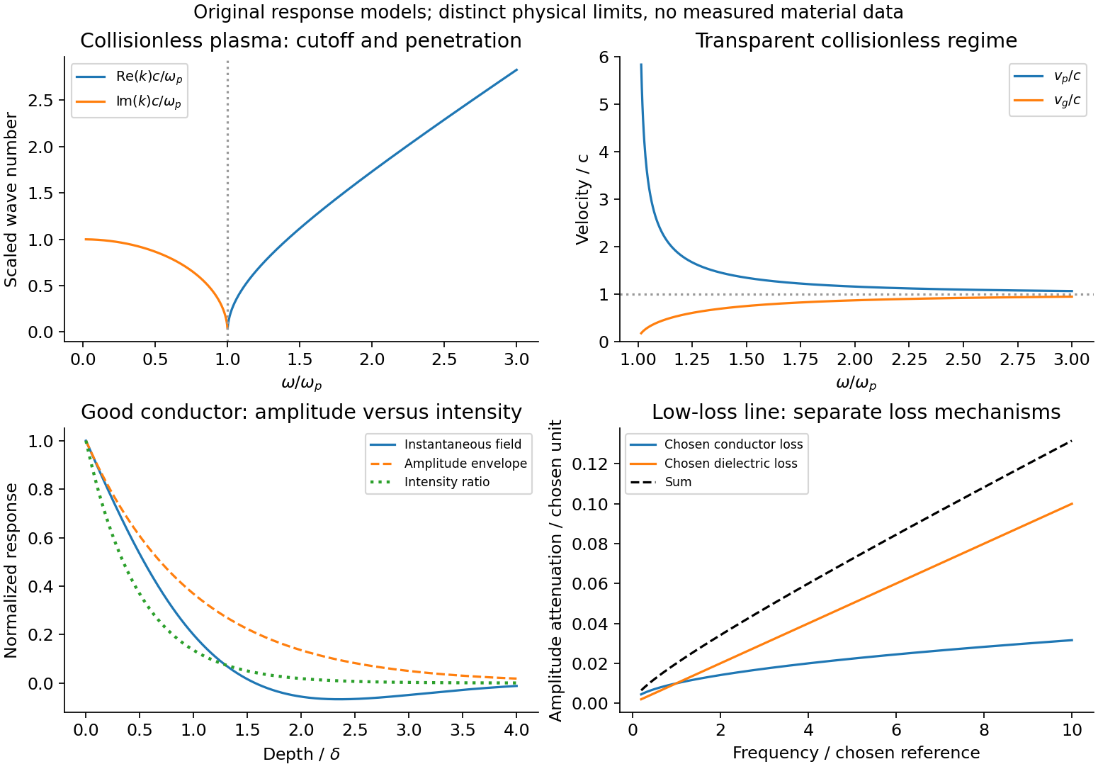
Conducting-wave propagation
. Chosen dispersion and decay models. Details.The vorticity of a fluid velocity field is . A vortex line is an integral curve tangent to that vector, not generally a particle path or streamline. Since , vorticity flux through successive cross-sections of a vortex tube is equal; a regular line cannot simply end inside the fluid. By Stokes's theorem, the tube strength is the circulationFor an inviscid barotropic fluid with conservative body force, Kelvin's circulation theorem conserves circulation around a material circuit. Under those assumptions vortex tubes move with the fluid. In three-dimensional incompressible ideal flow,stretching a material tube raises its vorticity as its cross-section shrinks. In two-dimensional incompressible flow there is no such stretching, so scalar vorticity is materially conserved. Constant viscosity adds a diffusion term ; baroclinicity and boundaries can also generate vorticity.
An ideal line vortex has and zero ordinary vorticity for , with its circulation concentrated in the singular core. Circular trajectories therefore do not imply nonzero local vorticity everywhere. A finite physical core removes the velocity singularity.
A freely rotating rigid body with no external torque conserves its inertial angular momentum and kinetic energy. In body-fixed principal axes, the Euler equations includeand cyclic permutations. The body can still change its orientation relative to its fixed angular-momentum vector; zero torque does not require every principal axis to remain fixed.
For a symmetric top, , . The axial rate is constant, and rotates in body coordinates with signed frequency . In space,Thus the symmetry axis precesses about fixed at rate and constant inclination. This body-frame and space-frame frequencies of free symmetric-top precession distinction avoids confusing two different frame-dependent rates. A sphere has no dynamically distinguished symmetry axis even though a chosen body marker rotates.
For a general body, rotations about the largest and smallest principal inertias are stable to small perturbations, while rotation about the intermediate inertia is unstable. With and rotation , linearization gives , showing exponential growth. This is torque-free motion, distinct from the gravity-driven precession of a supported gyroscope.
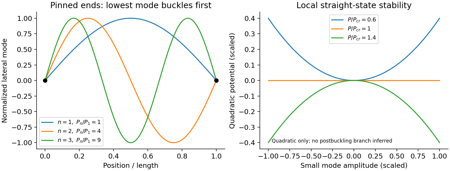
An Euler strut is a slender initially straight elastic column under axial compression. For a uniform bending stiffness and a small transverse displacement , the second-order potential energy under a conservative compressive load isThe bending term is positive; shortening releases load potential. Stationarity yields . Pinned ends impose and zero end bending moments, . Substitution of givesThe straight configuration loses stability first in the longest admissible bending mode. The second moment of area is geometric, not a mass moment of inertia. Boundary conditions matter: a fixed-free column has effective length , while fixed-fixed ends have effective length , changing the threshold by factors and . Slenderness, elastic material response, alignment and the weak bending direction must be checked. Imperfections produce bending before the ideal threshold, and a short column can yield or crush first. Linear buckling theory does not predict an unlimited deflection or a complete postbuckling curve.
The Reynolds number is , comparing inertial stress with viscous stress . Nondimensionalizing an incompressible Newtonian flow with velocity , length and pressure givesAt small Reynolds number inertia is negligible and a creeping-flow balance applies. At large Reynolds number the outer flow may be approximately inviscid, but thin no-slip boundary layers can still govern drag, separation and dissipation. A high Reynolds number permits turbulent motion without guaranteeing it; transition depends on geometry, disturbances and roughness.
Dynamically similar model experiments need matching geometry and relevant dimensionless parameters, including Reynolds number. If gravity, compressibility or surface tension matters, Froude, Mach or capillary-related parameters must also be matched. Testing linear pressure-flow or force-speed relations while varying , , viscosity and temperature is more informative than assigning one universal transition value to all apparatus.
stress describes internal force per area. A cut with unit normal has traction ; its normal component is and its remainder is shear traction. force balance constrains the stress divergence, while ordinary local angular-momentum balance makes the Cauchy stress tensor symmetric in a medium without body couples.
strain describes deformation rather than force. For small displacement gradients,The antisymmetric displacement-gradient part is a rigid rotation to first order and contributes no infinitesimal strain. Engineering shear strain is , so it must not be confused with the tensor component. stress has units of pressure; strain is dimensionless.
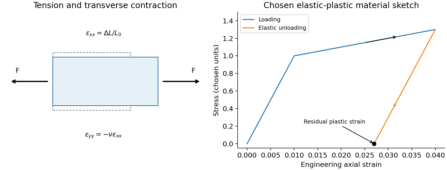
An isotropic linear elastic solid obeysTwo independent moduli are required. The shear modulus and bulk modulus must be positive for stability. Young's modulus and Poisson ratio satisfyFor a tensile specimen with free side faces, gives and . Pure shear gives ; hydrostatic loading gives . The incompressible limit has at finite shear stiffness, not vanishing shear resistance. Crystals can be anisotropic and need a fourth-rank elastic stiffness tensor instead of the isotropic two-constant law.
elastic deformation is recoverable on unloading; it need not remain linear at large strain. Beyond yield, irreversible rearrangements such as dislocation motion cause plastic strain, often followed by hardening. Ductile samples can neck before fracture; brittle failure has much less plastic deformation. Engineering stress uses initial area, while true stress uses the changing instantaneous area. A decreasing engineering stress during necking therefore need not mean that local true stress decreases. stress concentrations, flaws and loading geometry can determine failure before a uniform-material strength is reached. Viscoelastic materials also show rate dependence, creep and stress relaxation; their losses cannot be described by a static Hooke law alone.
A tensile test should measure force and gauge-length extension independently, correct machine compliance, align the grips, and control strain rate and temperature. Unloading distinguishes recoverable strain from a residual plastic extension. Separate shear or hydrostatic tests determine moduli that one axial measurement does not fix. Compression specimens need friction and buckling checks. Work per volume is ; the recoverable part is elastic energy, while a dissipative cycle produces a loss rather than creating energy. The original loading/unloading curve below is a chosen constitutive sketch, not measured material data.
For a fixed-composition simple compressible system, gives and . Equality of mixed derivatives yields . ThereforeFor one mole of ideal gas, , so . Reversible heat at fixed pressure gives , and consequentlyWith constant positive molar heat capacity, integrate from a reference state :If heat capacity varies, the last term must instead be . The reference ratios make the logarithms dimensionless. The following classical ideal-gas entropy limits test where the constant-heat-capacity expression remains applicable.
At fixed positive pressure, the extrapolated term tends to as . That prediction is not physically realistic for an equilibrium sample. The classical ideal-gas description with constant heat capacity cannot extend unchanged to absolute zero. A real substance generally undergoes phase changes, and quantum statistics and thermal freeze-out change its heat capacity and entropy. For a nondegenerate equilibrium ground state, the third law gives entropy approaching zero; residual ground-state degeneracy can give a finite residual value rather than this negative divergence. This is a breakdown of the extrapolation, not a violation of the third law by a real gas.
At fixed positive temperature, tends to as . This is a physically meaningful unbounded-volume limit for a fixed mole number: , so the number of accessible translational configurations grows without bound. For an ideal gas the entropy difference is at fixed temperature. No finite vessel reaches an infinite entropy, and at finite temperature is not a finite-volume one-mole state. The divergence is approached by dilution; it does not conflict with the third law, which concerns a different temperature limit.
Let two weakly coupled bodies exchange energy while their total energy is fixed. If body1 has , the number of compatible states is . Its most probable equilibrium division maximizes the logarithm, givingThis equal intensive quantity labels thermal equilibrium. With and thermodynamic ,Ordinary positive heat capacities make the entropy maximum locally stable. Particle numbers and volumes are held fixed during the exchange.
For a subsystem coupled to a large heat bath, the exact level weight is proportional to . Expanding the bath entropy gives . Normalization therefore givesThe Boltzmann form uses the reservoir limit; an arbitrary small isolated pair instead retains its exact bath state count. The degeneracy counts distinct subsystem microstates at the same energy, rather than adding another Boltzmann factor for the whole level.
In the two-level donor occupancy model, set the single bound-state energy to zero and the conduction representative to with degeneracy . Ignoring spin, its bound probability isThe measured model occupancy gives , sousing . The supplied occupancy and energy are rounded, so there is no reason to demand an exact nonrounded integer from that inference.
For , the excited-to-bound weight must be . Eliminate using the first point:The probability decreases monotonically from1 as toward as . The nonzero high-temperature limit follows from the stipulated finite effective degeneracy, not from a full continuum conduction-band calculation. A realistic band with energy-dependent density of states need not retain this two-level limit.
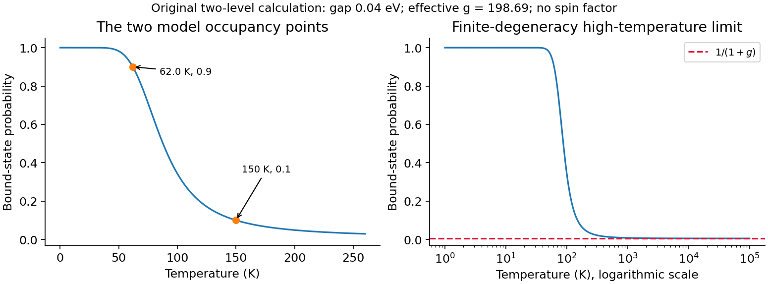
Donor occupancy
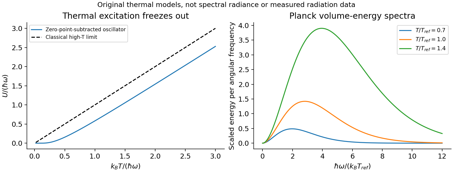
. Two-level model with both inferred temperature points. Details.For excitation energy , the geometric series gives the thermal partition function of a quantum harmonic oscillator with its zero-point energy subtracted:Thus at low temperature and approaches at high temperature. Restoring the zero-point term multiplies by and adds to , without changing the thermal occupation probabilities.
To count electromagnetic modes, put a large cavity in a periodic box of volume . One transverse polarization has wavevector-state density ; there are two independent polarizations. In the shell ,With , the electromagnetic mode density in a box becomesThe continuum expression is the large-cavity leading term; using standing-wave boundary conditions gives the same bulk count. Both photon polarizations must be included. This is density per angular frequency, not per ordinary frequency.
Each mode is an oscillator with zero photon chemical potential in thermal equilibrium. Multiplying its mean thermal energy by the mode density per volume gives the angular-frequency Planck energy densityAt small it reduces to the Rayleigh–Jeans result ; exponential suppression at high frequency prevents a divergent thermal energy. With ,The integral is the stipulated . This is a volume energy density, ; for isotropic cavity radiation the outward black-surface flux is , with . Distinguishing flux, spectral density and total volume energy avoids extra factors of , or .


The zeroth law of thermodynamics states the transitivity of thermal equilibrium: if two systems each equilibrate thermally with a third, they equilibrate with one another. A reproducible thermometric property can therefore label their temperature. Its empirical numerical scale is not itself the complete thermodynamic content; reversible heat-engine relations establish an absolute temperature scale.
The first law of thermodynamics expresses energy conservation. For a closed system, when is work done by the system. internal energy is a state function, while heat and work depend on the path. In reversible simple compressible motion, and ; an open system additionally needs the energies carried by transferred matter. An ideal gas can expand freely with and unchanged internal energy. The first law alone does not decide whether the reverse spontaneous process occurs.
The Second law of thermodynamics introduces entropy and restricts direction. For a reversible path, ; for an irreversible process the entropy balance includes nonnegative production. The entropy of an isolated system cannot decrease. In a cycle, the Clausius inequality is , using the appropriate boundary/reservoir temperatures. The Kelvin–Planck statement forbids a cyclic device whose sole effect is extracting heat from one reservoir and turning all of it into work; the Clausius statement forbids moving heat from cold to hot with no compensating effect. A refrigerator is allowed because it consumes work. A two-reservoir engine has , with equality in the reversible limit. Work may be fully dissipated as heat without contradicting this one-way restriction.
The third law of thermodynamics constrains low-temperature entropy. An equilibrium perfect crystal with a nondegenerate ground state approaches zero entropy as , fixing the conventional absolute entropy reference. Degenerate ground states or frozen nonequilibrium disorder require care when discussing residual entropy. Under regular equilibrium conditions the heat capacity must decrease sufficiently for to remain finite; a constant positive classical heat capacity cannot be extrapolated to zero temperature. The unattainability formulation states that absolute zero cannot be reached by a finite sequence of admissible cooling operations. These statements concern the limiting thermodynamic regime, rather than predicting that every substance stays in one classical phase during cooling.
The laws work together: conservation sets a device's energy budget, entropy production restricts the attainable budget, and constitutive equations give the properties of its working material. For fixed temperature and volume, Helmholtz free energy decreases toward equilibrium; at fixed temperature and pressure the corresponding potential is Gibbs free energy. Stable equilibrium, phase coexistence and Maxwell relations follow from these potentials with appropriate constraints. Calorimetry, mechanical-work measurements, thermometry and reversible-path comparisons test different parts of this framework. None of the laws by itself supplies a particular gas equation of state or microscopic heat capacity.
Articles by others on the same topic
There are currently no matching articles.