Past exam of the physics of atmospheres and oceans course of the University of Oxford / 2017 (A11048W1, C5)

Source paper: www.whatdotheyknow.com/request/oxford_physics_past_papers_2/response/2340696/attach/5/Physics%20Papers%202016.pdf?cookie_passthrough=1

Use $u$ as a spectroscopic wavenumber, in the same units throughout. Write the mass absorption coefficient of the absorbing species asHere $S$ is the spectral line strength, the integrated mass absorption coefficient; it is not the line-centre coefficient. If ${\kappa }_{\nu }$ has units ${\mathrm{m}}^2\mathrm{k}{\mathrm{g}}^{-1}$ and $\nu$ is in $\mathrm{c}{\mathrm{m}}^{-1}$, then $S$ has units ${\mathrm{m}}^2\mathrm{k}{\mathrm{g}}^{-1}\mathrm{c}{\mathrm{m}}^{-1}$. For absorber mass density ${\rho }_a$, the volume coefficient in Beer-Lambert law is ${\rho }_a{\kappa }_{\nu }$.

Lifetime broadening. Finite lifetimes of the upper and lower states destroy optical coherence, even for an isolated molecule. Exponential coherence decay gives a Lorentzian line shape. For population decay rates ${\Gamma }_u,{\Gamma }_l$ and no extra dephasing, its wavenumber half-width is $({\Gamma }_u+{\Gamma }_l)/(4\pi c)$, with $c$ expressed in the length unit reciprocal to $\nu$. This sets a natural linewidth and can matter at extremely low collision rates; it is generally much smaller than atmospheric collisional or thermal widths.

Thermal Doppler broadening. A Maxwell-Boltzmann distribution of molecular line-of-sight velocities givesThis Gaussian distribution has a $1/e$ half-width ${\Delta }_D$, determined by absorber molecular mass $m_a$ and temperature. It is especially relevant in the rarefied upper atmosphere, where collisions are infrequent.

Pressure broadening. Collisions perturb transition frequencies and phases. In the impact regime, exponential phase decorrelation givesHere ${\Delta }_L$ is the half-width at half maximum, proportional to the coherence-destroying collision rate. It depends on perturber density, molecular collision properties, and temperature; it is often parameterized by ${\Delta }_L\propto p(T_{\ast }/T{)}^{n_T}$ for a specified broadener. It dominates much of the dense lower atmosphere. The Lorentzian line shape has algebraic $\delta {\nu }^{-2}$ wings, whereas the Doppler profile has rapidly decreasing Gaussian wings. Where both mechanisms matter, their convolution is a Voigt profile. A pure pressure-broadened profile should not be extrapolated to arbitrarily low pressure while discarding the finite Doppler core.

Let $m$ be the absorber mass path along a ray. If the spectral line profile is independent of position, Beer-Lambert law gives ${\mathfrak{T}}_{\nu }(m)=e^{-m{\kappa }_{\nu }}$. A finite-band mean and the line's equivalent width are respectivelyWhen the band contains all significant absorption, ${\int }_{\mathcal{B}}{\mathfrak{T}}_{\nu }d\nu \simeq \Delta {\nu }_{\mathcal{B}}-E$. An unqualified integral of transmission over the entire infinite line domain diverges because transmission tends to one far from line centre; $E$ is the finite and physically useful line deficit.

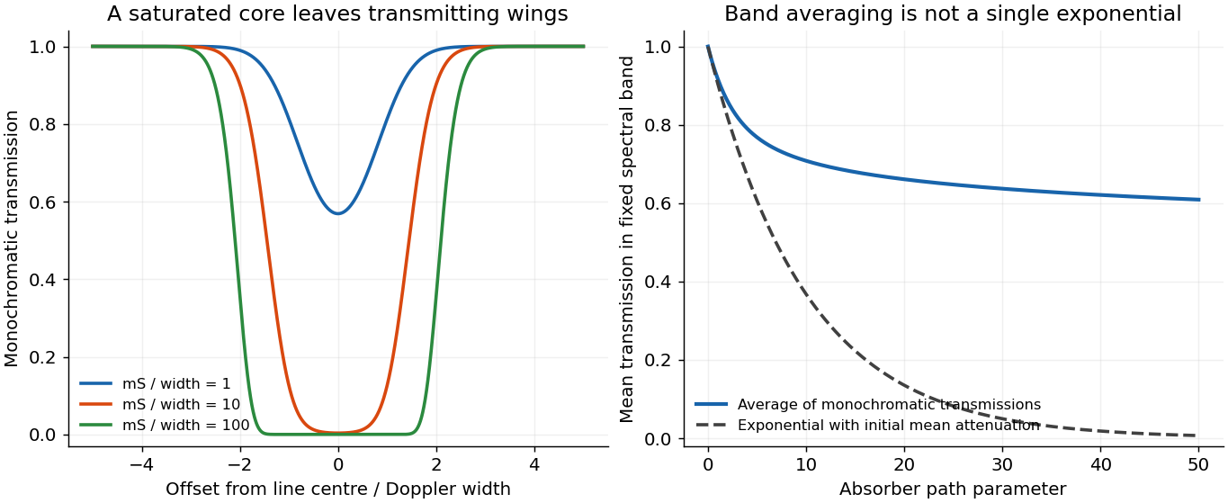
This is nonexponential band transmission: each monochromatic transmission is exponential, but their average generally is not. Differentiating with respect to mass path givesMore decisively, define the absorption coefficient averaged over the transmitted spectrum byThen $\boxed{a_{\mathrm{eff}}^{\prime }(m)=-{\mathrm{Var}}_m(\kappa )\le 0}$. The core saturates first and the surviving radiation increasingly samples weakly absorbing wings. The effective attenuation per additional mass therefore decreases. Jensen's inequality also gives $\overline{\mathfrak{T}}\ge e^{-m⟨\kappa ⟩}$, with equality for a spectrally constant coefficient. Thus the band transmission decays more slowly than the exponential with its initial mean attenuation.

The corresponding curve of growth has $E(m)\simeq mS$ for an optically weak line, and sublinear growth after saturation. For the Gaussian profile, with ${\tau }_0=mS/(\sqrt{\pi }{\Delta }_D)\gg 1$, absorption extends to $|\delta \nu |\simeq {\Delta }_D\sqrt{\log {\tau }_0}$, so $E\sim 2{\Delta }_D\sqrt{\log {\tau }_0}$. For a strongly saturated pure Lorentz profile the wings instead give $E\sim 2\sqrt{mS{\Delta }_L}$. These asymptotes apply while the line remains isolated and its important wings remain within the range where the assumed profile and nearly constant Planck function are appropriate. The integrated absorption is not an exponential either: $E^{\prime }>0$ and $E^{\prime \prime }\le 0$.

For the single-line greenhouse deficit, use hydrostatic balance, fixed surface pressure $p_s$, constant gravity $g$, and the dry adiabatThe gas constant and specific heat refer to the background gas. Let ${\mu }_d=\cos \tilde{\theta }>0$ be the supplied effective ray cosine. The vertical optical depth and slant transmittance from level $p$ to space areThis permits pressure-dependent line widths. With local thermodynamic equilibrium, negligible infrared scattering, a black thermal surface, and no incident thermal radiation from space, the formal radiative transfer solution isThe weights add to one. Subtract the transparent-surface radiance and put $B(p)=B_{{\nu }_0}(T(p))$, using the narrow-line approximation only in the line deficit. Define its pressure-dependent equivalent widthApproximating each hemispheric flux by $\pi$ times the effective-ray radiance preserves the black-surface flux. The outgoing longwave flux is thereforeIntegration by parts gives the particularly transparent formBoth boundary terms vanish: $E(0,q)=0$ and $B(p_s)-B(p_s)=0$. The dry adiabat and monotonic Planck function give $dB/dp>0$. Atmospheric emission replaces part of the warm surface radiation by emission from cooler levels, reducing emission to space for a specified $T_s$. The inequality is strict when opacity occurs over a nonzero range with temperature contrast; an isothermal absorbing layer at the surface temperature would not produce such a contrast.

For a spherical planet the mean absorbed instellation is $F_{\ast }=(1-\alpha )L_{⊛}/4$. The required global energy balance isConsequently every equilibrium of this model has $T_s\ge T_{\mathrm{bare}}=[(1-\alpha )L_{⊛}/(4{\sigma }_{\mathrm{SB}}){]}^{1/4}$, with strict warming when $D>0$. At fixed temperature profile, increasing $q$ increases $E$ and hence $D$. This argument does not assume that the greenhouse gas changes the stellar-band albedo, surface pressure, or background thermodynamics; those are held fixed. For sufficiently broad or overlapping saturated wings the full frequency-dependent Planck function must replace the narrow-line approximation.

Take a weak line in the radiative sense: the integrated slant optical depth is small wherever absorption materially contributes, not merely a small greenhouse-gas mass mixing ratio. Normalize every local spectral line profile so that $\int {\kappa }_{\nu }(p)d\nu =S$, with the line strength independent of pressure and, as stipulated, temperature. Keep a finite Doppler or natural core, or a Voigt profile, so that a pressure-only zero-width core at the top does not invalidate a uniform optical-depth expansion. The line must also be narrow enough to use $B_{{\nu }_0}$ across it.

To first order,Thus the detailed normalized line shape drops out, even if its width varies with pressure. Substituting in the deficit in c givesThe neglected term is second order when the relevant squared optical depths are integrable and uniformly small. A very narrow saturated line need not be weak simply because $q\ll 1$. More generally the displayed first-order integrated limit follows from the finite integrated opacity even if an idealized line centre makes a pointwise expansion nonuniform; a finite physical core is the straightforward sufficient assumption.

For an explicitly perturbative temperature estimate, evaluate the bracket at $T_{\mathrm{bare}}$:At fixed $p_s,g,q,S$ and radiative conditions, increasing $\kappa =R_b/c_{p,b}$ makes every level $0<r<1$ cooler relative to the surface, enlarging the bracket and the warming. Increasing $c_{p,b}$ at fixed $R_b$ has the opposite effect. The limit $\kappa \to 0$ is isothermal and gives zero line-induced deficit. A change of background molecular mass alone need not change this leading result: for ideal gases with the same active degrees of freedom, $R_b$ and $c_{p,b}$ scale together and their ratio is unchanged. Comparing only the height-coordinate lapse rate $g/c_{p,b}$ would miss that the absorber column is naturally a pressure-coordinate quantity.

Below cloud base, an initially unsaturated closed parcel expands as ambient pressure falls. In the absence of heat exchange its temperature falls approximately at the dry adiabatic lapse rate $g/c_{p,d}$. Its vapour mixing ratio is conserved, but its saturation mixing ratio decreases strongly as it cools. Hence relative humidity rises until the lifting condensation level is reached. The density normally decreases through expansion; the environmental profile determines the parcel's buoyancy and thus whether ascent can continue.

Near saturation, slight atmospheric supersaturation permits suitable cloud condensation nuclei to activate. Köhler theory describes the competition between curvature, which raises equilibrium vapour pressure, and dissolved solute, which lowers it. Cooling generates supersaturation, while condensation onto the new droplets consumes it. Their balance normally keeps in-cloud relative humidity close to, but not identically at, saturation. The activated droplet number depends on the aerosol population and the maximum supersaturation produced by the ascent.

Above cloud base, condensation lowers the vapour content and raises the liquid-water content. The latent heat released partly offsets expansion cooling, so the moist adiabat has a smaller lapse-rate magnitude than the dry one. In a dilute approximation,A closed adiabatic parcel conserves total water $q_t=q_v+q_l$ and approximately its moist entropy; retaining condensate makes this a reversible-cloud idealization, rather than a precipitating pseudoadiabat. In a shallow cloud, the saturation-mixing-ratio decrease and slow density variation yield nearly constant condensation per height, so liquid-water content is approximately linear above base. Once activation is complete, assuming nearly fixed droplet number per volume gives increasing droplet size as condensate accumulates. Entrainment, continued activation, collision-coalescence and atmospheric precipitation can all violate that simplified description; they are excluded from the stated retrieval model.

Using the adiabatic cloud droplet moments, define $N=\int n(r)dr$ and the mean volume radius by $r_v^3=N^{-1}\int r^{3}n(r)dr$. Summing the liquid mass of spherical droplets givesTherefore, with the shallow-cloud liquid-water content $w=c_{w}h$,The growth is $h^{1/3}$ at fixed number concentration, and the radius scales as $N^{-1/3}$ at fixed water content. The dimensions are consistent: $c_w$ has units $\mathrm{kg}{\mathrm{m}}^{-4}$, so $c_{w}h/({\rho }_{w}N)$ has units ${\mathrm{m}}^3$. The formula is a third-moment radius; a monodisperse distribution is not required. Fixed $N$ per volume is the shallow-cloud approximation, not exact conservation of number per parcel volume during an arbitrarily deep expansion.

Let $r_s^2=N^{-1}\int r^{2}n(r)dr$. The effective droplet radius and shape factor give $r_e=r_v^3/r_s^2$ and $k^{1/3}=r_v/r_e$, so $r_s^2=k^{1/3}{r}_v^2$. If the extinction efficiency is approximately independent of droplet size over the distribution,For visible wavelengths and droplets large compared with the wavelength, geometrical optics makes $Q_{\mathrm{ext}}\simeq 2$ a useful approximation. Retaining it as the specified constant, and taking $N,k,c_w$ constant over the cloud,The $3/5$ comes from integrating $h^{2/3}$; replacing the whole cloud by its cloud-top extinction would incorrectly omit it. The effective-radius relation treats the distribution shape through $k$, without assuming all droplets have the same size. Liquid phase, negligible vertical variation in that shape factor, and negligible departures from the adiabatic water profile are essential assumptions.

In the adiabatic cloud droplet number retrieval, the independently retrieved liquid-water path fixes the geometrical thickness in the adiabatic model:Define $C_c=(3/5)\pi Q_{\mathrm{ext}}{k}^{1/3}[3c_w/(4\pi {\rho }_w){]}^{2/3}$. Since ${\tau }_c=C_c{N}^{1/3}{H}^{5/3}$, eliminating $H$ givesUse SI units to obtain $N$ in ${\mathrm{m}}^{-3}$, then divide by $10^6$ for $\mathrm{c}{\mathrm{m}}^{-3}$. The sensitivity is substantial: $d\log N=3d\log {\tau }_c-(5/2)d\log W+(1/2)d\log c_w-d\log k-3d\log Q_{\mathrm{ext}}$. Thus a numerical retrieval additionally needs the adiabatic condensation coefficient, shape factor and extinction efficiency. A nonadiabatic water profile, mixed phase, horizontal inhomogeneity or a biased water-path retrieval can produce a large number-concentration bias.

Denote aerosol optical depth by ${\tau }_a$ to distinguish it from cloud optical depth. Retrieve $N$ as in d, collocate it with ${\tau }_a$, and estimate an aerosol-to-droplet susceptibilityA regression should control for water content, updraught and cloud regime; aerosol optical depth is not itself a direct measurement of activated nuclei. For an approximately constant $s_a$ over a factor two in aerosol, $N_2/N_1=2^{s_a}$.

Integrate the supplied cloud albedo susceptibility rather than treating a finite doubling as infinitesimal:For a small response, $\Delta A\simeq A_1(1-A_1)s_a\log 2/3$. If $F_{\mathrm{sw}}$ is the appropriate mean incoming shortwave flux and $f_c$ the fraction of the scene occupied by these clouds, the leading top-of-atmosphere perturbation, positive downward, isThe two transmissions account approximately for the atmosphere above the cloud and may be absorbed into an effective illuminating flux. In the simplest global transparent-overburden estimate $F_{\mathrm{sw}}=L_{⊛}/4$. Positive $s_a$ gives increased reflection and negative shortwave forcing, the Twomey effect. Numerical forcing cannot be determined from the given susceptibility alone: it needs baseline albedo, cloud fraction, illumination and an empirically constrained $s_a$. Humidity swelling, cloud contamination of aerosol retrievals and common meteorological influences can create spurious correlations. Changes in cloud amount, water path or lifetime are additional adjustments, not the fixed-water Twomey term derived here.

Put the rigid lid at $z=0$, the interface at $z=-h(x,y,t)$ and ${\rho }_1={\rho }_0-\Delta \rho$. Assume hydrostatic vertical balance and a resting deep layer. Its pressure is $p_2=C-{\rho }_{0}gz$, with horizontally uniform $C$. Pressure continuity at the interface then fixes the upper-layer pressure:Hence its horizontal pressure gradient at fixed $z$ is ${\nabla }_h{p}_1=\Delta \rho g{\nabla }_{h}h$, independent of depth. Taking the horizontal momentum equation and a vertically uniform upper-layer velocity givesThe exact density denominator for upper-layer acceleration is ${\rho }_1$; the familiar ${\rho }_0$ denominator is the small-density-contrast Boussinesq approximation. The restoring pressure is weaker than for a free surface because only the density difference contributes.

The horizontal shallow-layer equations use the vertical component of planetary rotation: $f=2\Omega \sin \phi$. Thus the source's vector notation is interpreted as the projected vector $f\mathbf{k}$ after the traditional approximation. Taking the full magnitude $2\Omega$ as a midlatitude Coriolis parameter would discard the latitude dependence. Together with layer-volume conservation, the model has ${\partial }_{t}h+{\nabla }_h\cdot (h\mathbf{u})=0$.

Both descriptions are depth-averaged hydrostatic shallow-layer models. In a one-layer free-surface shallow water equations, a homogeneous layer overlies a rigid bottom and its upper surface moves. Surface elevation changes give a restoring acceleration based on full gravity $g$, with external-wave speed $\sqrt{g{H}_0}$. Barotropic coastal storm surges, long surface gravity waves or a basin seiche are examples.

In the rigid-lid reduced gravity model, the movable boundary is a density interface beneath the active upper layer, while the much deeper lower layer remains at rest. The internal interface mode instead has speed $\sqrt{g^{\prime }{h}_0}$ and represents, for example, thermocline displacements and an upper-ocean baroclinic eddy. The mathematical shallow-water form is retained with $g$ replaced by $g^{\prime }$ and with the appropriate interface-depth convention. A freely moving two-layer surface would support both external and internal modes; the rigid lid filters out the fast external mode, and the resting abyss removes its independent dynamics.

Write $h=h_0+\eta$, with small interface displacement $\eta$ and horizontal variation scale $L$. The geostrophic pressure-Coriolis balance givesSubtracting the uniform reference state and the mass-conserving linear potential-energy term, the perturbation energy densities per unit horizontal area areThereforeThe internal deformation radius $L_R$ is the distance an internal gravity wave travels in an inverse-Coriolis time. Balanced broad disturbances $L\gg L_R$ mainly store available potential energy; balanced fine structures $L\ll L_R$ require relatively large kinetic energy. This scale result presupposes small Rossby number $U/(|f|L)$; reducing the length at fixed displacement eventually violates geostrophy. It does not say an initially resting small-scale height perturbation already has that large kinetic energy: such a perturbation undergoes geostrophic adjustment.

Let $K=(k^2+l^2{)}^{1/2}$ and $c=\sqrt{g^{\prime }{h}_0}$. The three branches areFor nonzero $K$ and $f$, the zero-frequency mode is stationary geostrophic flow, with $f\mathbf{k}\times \mathbf{u}=-g^{\prime }\nabla \eta$ and zero horizontal divergence. It carries the linear potential-vorticity disturbance. There is no Rossby-wave propagation on a constant-$f$ plane; a varying Coriolis parameter would be needed for that.

The other two branches are oppositely phased inertia-gravity waves. Their phase-speed magnitude and radial group velocity are $|\omega |/K=\sqrt{c^2+f^2/K^2}$ and $|\partial \omega /\partial K|=c^{2}K/\sqrt{f^2+c^2{K}^2}$. When $K{L}_R\gg 1$, gravity dominates: $|\omega |\simeq cK$ and the waves are approximately nondispersive, with both speeds approaching $c$. When $K{L}_R\ll 1$, rotation dominates: $|\omega |\simeq |f|+c^2{K}^2/(2|f|)$, the frequency approaches the inertial frequency and the group velocity tends to zero. The large long-wave phase speed is not a large signal speed.

Without rotation the propagating branches become nondispersive gravity waves, $\omega =\pm cK$, and the stationary branch is a nondivergent vortical velocity disturbance rather than a finite-pressure geostrophic balance. At $K=0$, the modes reduce to constant interface height and spatially uniform inertial oscillations. The wave branches have zero linear potential-vorticity perturbation; it is the stationary branch that retains the initial potential vorticity.

A numerical scale estimate requires a reference ocean density and latitude not specified exactly. Taking ${\rho }_0\simeq 1025\mathrm{kg}{\mathrm{m}}^{-3}$, $g\simeq 9.81\mathrm{m}{\mathrm{s}}^{-2}$ and a representative midlatitude $|f|\simeq 10^{-4}{\mathrm{s}}^{-1}$ givesFor a small-amplitude interface displacement of scale $L=1\mathrm{km}\ll L_R$, gravity drives rapid horizontal acceleration and radiates most of the displacement in inertia-gravity waves. The gravity adjustment time is $L/c\sim 8$ minutes, much shorter than $1/|f|\sim 2.8$ hours. A weak balanced remnant remains in an unbounded inviscid adjustment problem; energy is carried away by waves, not dissipated merely by geostrophic adjustment.

For $L=100\mathrm{km}\gg L_R$, rotational adjustment produces a largely retained interface displacement with a geostrophic current. Wave emission and inertial oscillations accompany the adjustment, but the balanced structure is much more important. To quantify that distinction under an initially resting, linear single-Fourier-component assumption, potential-vorticity conservation givesThis is about $0.002$ for the kilometre scale and $0.95$ for the hundred-kilometre scale. These fractions use $L$ as an inverse wavenumber scale, not a full wavelength, and are illustrative rather than unique predictions for an unspecified disturbance or bounded basin.

For a unit mass of ideal gas, the first law of thermodynamics in enthalpy form is $\delta Q=c_{p}dT-vdp$. A reversible adiabatic displacement has $\delta Q=0$, and the ideal gas law gives $v=RT/p$. ThusThe atmospheric profile approaches this dry adiabat when convection efficiently mixes potential temperature and there is no condensation or other strong diabatic source. The first law by itself determines a parcel path, not every possible environmental temperature profile; the convective mixing assumption is needed. Hydrostatic balance gives the corresponding height lapse rate $dT/dz=-g/c_p$.

For rigid linear molecules with translation and rotation active but vibration frozen, the molecular heat capacities are $C_V=(5/2)R_u$ and $C_P=(7/2)R_u$, hence $R/c_p=2/7$. Earth is dominated by the diatomic gases nitrogen and oxygen. Mars is dominated by carbon dioxide, which is triatomic but linear and has the same two rotational degrees of freedom. In the rigid-molecule approximation it therefore has the same ratio. The value is not exact for carbon dioxide when its bending vibrations contribute appreciably to heat capacity, and variable heat capacities give a nonconstant dry-adiabatic exponent. Here $\gamma$ denotes $R/c_p$, not the distinct adiabatic index $c_p/c_v$.

Assume a plane-parallel atmosphere in local thermodynamic equilibrium, negligible infrared scattering, a black surface, and surface temperature equal to the adjacent air temperature. For a specified ray, let $\mathfrak{T}$ be its transmittance from a level to space, increasing from ${\mathfrak{T}}_0$ at the surface to one at the top. The formal radiative transfer solution isUsing ${\mathfrak{T}}_0+{\int }_{{\mathfrak{T}}_0}^{1}d\mathfrak{T}=1$ yieldsThis expresses absorption and re-emission together: opacity does not simply remove surface radiation without adding atmospheric radiation. An absorber close to a thermally coupled surface has nearly the same Planck function as that surface, so $B-B_0$ is small. Its emission nearly compensates the surface radiation it absorbs, giving weak radiance sensitivity to near-surface concentration. In an exactly isothermal atmosphere at surface temperature, $L=B_0$ for every optical depth, a concrete example of complete concentration ambiguity in this thermal measurement. Finite surface emissivity, reflection, scattering or a surface-air temperature discontinuity would require additional terms.

A hydrostatic pressure interval contains $dp/(gM)$ moles of background gas per area. Its absorbing column is $x(p)dp/(gM)$, so for a nadir rayThe assumed Planck-temperature power and dry adiabat give $B(p)/B_0=[T(p)/T_0{]}^{3.5}=p/p_0$. To first order in optical depth, $-d\mathfrak{T}\simeq d\tau$, and the radiance solution becomesFor a uniform mixing ratio this also evaluates to $L\simeq B_0[1-k_{0}x{p}_0/(6gM)]$. Its total optical depth is ${\tau }_0=k_{0}x{p}_0/(2gM)$, so the deficit is $B_0{\tau }_0/3$.

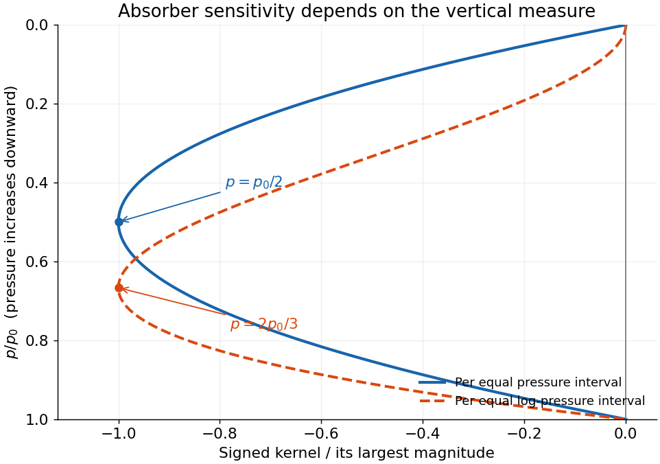
A pressure-resolved perturbation defines the infrared absorber sensitivity kernel by $\delta L=\int K_p(p)\delta x(p)dp$, withIt is zero at the top, negative in the interior, and zero again at the surface. The magnitude is largest where $d{K}_p/dp=0$, namelySign and coordinate qualification. Literally the maximum of the signed kernel is zero at the endpoints; $p_0/2$ is its minimum and the maximum of its absolute value. The derivative with respect to a single vertically uniform $x$ is the integrated constant $-k_0{B}_0{p}_0/(6gM)$ and has no pressure location. For equal-width logarithmic pressure perturbations the kernel is instead $K_{\log p}=p{K}_p$ and its magnitude peaks at $2p_0/3$. The stated pressure-interval convention is therefore essential.

The low top-of-atmosphere sensitivity reflects the small pressure-broadened absorption coefficient and small molecular column per $dp$ there; the low surface sensitivity reflects small thermal contrast. The printed phrase that temperature decreases with pressure reverses the actual stipulated relation: with positive exponent, temperature decreases as pressure decreases upward. The derivation uses the explicit adiabatic formula.

Take an isothermal hydrostatic reference atmosphere, ${\rho }_0(z)={\rho }_s{e}^{-z/H}$, and linearize about rest. The horizontal acceleration and pressure-gradient force retain the equatorial Coriolis parameter $f\simeq \beta y$, with $\beta =2\Omega /a$. The traditional approximation retains only its vertical component. Quadratic perturbation advection is neglected. The vertical acceleration is balanced by perturbation buoyancy and pressure gradient after removing the reference hydrostatic balance.

The continuity constraint is the anelastic approximation, $\nabla \cdot ({\rho }_0\mathbf{u})=0$, giving $u_x+v_y+w_z-w/H=0$. It retains stratification-driven expansion while filtering acoustic density fluctuations. It is therefore not the full compressible continuity equation. Adiabatic displacement in a stably stratified background gives $b_t+N^{2}w=0$, with $N$ the Brunt–Väisälä frequency; upward displacement develops restoring negative buoyancy.

Pressure convention matters. With the entropy-buoyancy equation just described, a consistent reduced-pressure form writes the pressure acceleration as $-\nabla \Phi$, where $\Phi =p^{\prime }/{\rho }_0$. Its vertical term is $-{\partial }_z(p^{\prime }/{\rho }_0)$, not simply $-{\rho }_0^{-1}{p}_z^{\prime }$. The original source explicitly specifies variable ${\rho }_0(z)$ but prints the latter. Those differ by $p^{\prime }/({\rho }_{0}H)$, so the two cannot silently be equated. Parts b and c display the consequence and then solve the explicitly corrected reduced-pressure model that yields the requested wave equation. This is a mathematical inconsistency in the printed set, not missing source material.

First check the printed equations literally. Set $v=0$ and use ${\rho }_0^{\prime }/{\rho }_0=-1/H$. Differentiating continuity in time and using horizontal momentum givesVertical momentum and buoyancy give $w_{tt}+N^{2}w=-p_{zt}/{\rho }_0$. Combining them therefore yieldswhich differs from the requested equation. The factor two arises when differentiating both ${\rho }_0$ and $w_z-w/H$. Keeping variable density in continuity while treating it as constant during that differentiation would be inconsistent.

For the intended anelastic reduced-pressure Kelvin wave, make the explicit correction $w_t-b+{\Phi }_z=0$, while $u_t+{\Phi }_x=0$ and $\Phi =p^{\prime }/{\rho }_0$. Continuity then gives ${\Phi }_{xx}=w_{zt}-w_t/H$, and vertical momentum gives $w_{tt}+N^{2}w=-{\Phi }_{zt}$. Cross differentiation now producesThis proves the advertised equation for the corrected model, without claiming it follows from the incompatible printed set.

A concrete counterexample makes the distinction testable. In nondimensional units $H=N=k=1$, take $m=0$, $\omega =2/\sqrt{5}$ and $w=e^{z/2}{e}^{i(x-\omega t)}$, multiplied by its Gaussian meridional envelope. This satisfies the last boxed wave equation, but substitution into the literal printed-system wave operator gives $-2w/5\ne 0$. No choice of accompanying pressure and horizontal velocity can then make it a solution of all five printed equations. Conversely, the literal operator has vertical factors $e^{z/H+imz}$ and dispersion ${\omega }^2=N^2{k}^2/(k^2+m^2)$; its scaling is different from the requested half-scale-height factor.

Work with the explicitly corrected reduced-pressure system in b. Write $d=1/(2H)$ and use the complex wave amplitude, taking real parts at the end. The vertical factor satisfies $({\partial }_z^2-H^{-1}{\partial }_z)w=-(m^2+d^2)w$, so the wave equation givesFor a Kelvin wave, continuity, zonal momentum and the buoyancy equation then determine all polarizations:In particular $u,w,b,\Phi$ have amplitude proportional to $e^{z/(2H)}$, whereas pressure $p^{\prime }$ has amplitude proportional to $e^{-z/(2H)}$. Directly substituting these expressions into vertical momentum gives ${\Phi }_z=-i\omega (m^2+d^2)w/k^2=i(\omega -N^2/\omega )w$, verifying both the sign and the dispersion relation.

Meridional momentum is $\beta yu+{\Phi }_y=0$. Since $\Phi =cu$, it integrates to a Gaussian $\exp [-\beta y^2/(2c)]$. ThusThe eastward intrinsic branch $c>0$ is selected by decay away from the equator; choosing $c<0$ would make the meridional amplitude grow without bound. Although the squared dispersion relation has both frequency signs, a meridionally trapped Kelvin wave has this one phase-propagation direction.

For short vertical wavelengths, $m^2\gg k^2+d^2$, so ${\omega }^2\simeq N^2{k}^2/m^2$, $c\simeq N/|m|$ and $L_D^2\simeq N/(\beta |m|)$. The wave is a slowly oscillating, hydrostatic internal gravity wave with strong vertical variation and relatively narrow trapping. Here $u\simeq -(m/k)w$ and $p^{\prime }/{\rho }_0\simeq -(\omega m/k^2)w$; the buoyancy expression above remains valid.

For long vertical wavelengths, $|m|\ll \sqrt{k^2+d^2}$, the exact limiting speed is $c=N/\sqrt{k^2+d^2}$. To obtain the stated height-controlled limit also requires long horizontal wavelength, $|k|H\ll 1$. With both $|m|H\ll 1$ and $|k|H\ll 1$,The finite density scale height prevents the hydrostatic $1/|m|$ phase speed from diverging as $m\to 0$. The polarizations tend to $u\simeq -iw/(2Hk)$, $\Phi \simeq -iNw/k$ and $b\simeq -iNw/(2Hk)$. Long vertical wavelength alone at fixed large $kH$ would not justify $c=2NH$. In the opposite horizontally short limit the frequency approaches $N$ instead. The growth $e^{z/(2H)}$ compensates decreasing reference density in wave-energy density; a radiating wave train is a local modal description, not a finite-total-energy eigenfunction over an infinite vertical domain.

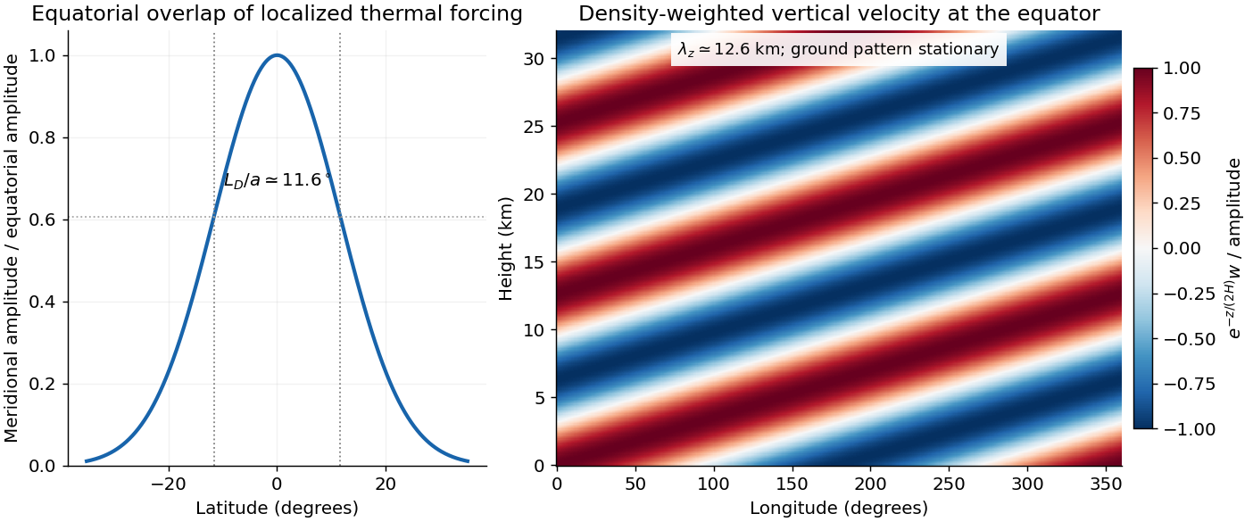
Apply the intended, corrected dispersion relation in c. A uniform mean zonal wind gives ${\omega }_{\mathrm{ground}}=\hat{\omega }+kU$. Stationarity with $U=-20\mathrm{m}{\mathrm{s}}^{-1}$ therefore requires eastward intrinsic phase speed $\hat{\omega }/k=-U=20\mathrm{m}{\mathrm{s}}^{-1}$. With $k=1/a$,The period determines $\Omega =2\pi /(24.4\times 3600\mathrm{s})$ and $\beta =2\Omega /a\simeq 4.21\times 10^{-11}{\mathrm{m}}^{-1}{\mathrm{s}}^{-1}$. Hence

A storm within roughly $12^{\circ }$ of the equator has substantial projection on the Gaussian mode. There is no sharp latitude cutoff: $|y|=L_D$ gives amplitude $e^{-1/2}$ and the $1/e$ amplitude latitude is about $16.4^{\circ }$. Forcing outside that core has progressively weaker overlap.