Original solutions to past examinations of the topics in fluid mechanics course of the University of Oxford.
Solutions to all three questions of the topics in fluid mechanics course of the University of Oxford examination, sat on 9 June 2023. Source: original released PDF, inclusive bundle pages 329–334; paper pages 1–6. All 24 lettered or Roman-numbered leaves across the three questions are covered. The original PDF labels the final part of Question 1 as (c), which is the hierarchy used here.
Take positive away from the wall into the liquid, and write for atmospheric pressure. For a constant-mass density Newtonian fluid, the two-dimensional Navier-Stokes equation and continuity equation areThe stationary wall imposes the no-slip boundary condition and no-penetration boundary condition, at . For a flat free surface with negligible air shear stress, the stress boundary condition is , at ; the kinematic boundary condition is there.
For steady flow independent of , these equations give , and . Two integrations and the boundary conditions give the uniform gravity-driven Newtonian film:Its surface velocity is , while its mean velocity is .
Define the aspect ratio and the thickness-based Reynolds number byUse the nondimensionalizationThe small transverse velocity scale follows from incompressibility. Dropping stars, the base fields become and . Before subtracting the base state, the dimensionless Navier-Stokes equation readsFor example, division of the downslope momentum equation by makes the inertial coefficient and the pressure gradient coefficient . The transverse equation has been divided instead by after using its smaller velocity scale; this gives the displayed coefficient.
Now substitute , , . Since , , and the base fields have no or dependence, subtraction givesThese are nonlinear equations for the deviations; small amplitude has not been assumed. The later asymptotic expansion takes as , or more generally requires the retained inertial correction to remain small.
The two wall boundary conditions areDefine the capillary parameter for a falling filmRetain in the long-wave approximation. Thus surface tension is retained in the leading normal stress balance even though geometric slope corrections are small. For in the rescaled coordinates, the dimensional surface slope is .
The three free surface boundary conditions, accurate through , areThe first is the kinematic boundary condition; the second is the zero tangential traction condition. For the third, the dimensional liquid-side pressure is, to the required order,Division by gives in dimensionless variables. Subtracting gives the stated perturbation condition. The additional slope-times-shear contribution to normal stress vanishes at this order because the tangential traction is zero. The omitted geometric and tangential-stress corrections are under this ordering.
Use an asymptotic expansion at fixed , evaluating the boundary conditions at the instantaneous . At leading order, the downslope equation gives . The wall condition and the surface condition implyHere denotes the total leading velocity, to distinguish it from the dimensional scale . The continuity equation and wall impermeability then giveThe transverse momentum equation gives . The normal stress condition therefore yieldsThe leading volume flux per unit width is . Consequently mass conservation gives . This relation eliminates inside the first inertial correction:Set . The downslope equation and boundary conditions areTwo integrations giveThe pressure correction is not needed for this calculation because its downslope pressure gradient enters only at .
Integrating the total velocity across the film givesIndeed the three inertial polynomial terms integrate to . Integrating the continuity equation and using the kinematic boundary condition gives . Hence the Benney equation isNormal gravity smooths height variations on the upper side of the slope, while the inertial correction can amplify them. Surface tension suppresses sufficiently short wavelengths.
For an inverted falling film, keep directed from the solid into the liquid. The downslope component of gravity is unchanged, but its normal component is now positive. Thus the hydrostatic pressure changes from to . The resulting Benney equation isOnly the normal-gravity contribution changes sign; the surface tension and inertial contributions retain their signs.
Define . The linearization about givesThe Galilean transformation , has and . It removes the leading advection, leavingFor a normal mode proportional to , the second and fourth derivatives contribute and . The dispersion relation is thereforeFor and , the unstable wavenumbers satisfy . In the laboratory coordinates, the temporal exponent is , so this linear stability calculation predicts growth together with downslope transport at dimensionless speed .
For , maximize the growth rate over real wavenumbers. Its derivative is , soThe second derivative at either nonzero maximizer is . If , there is no positive growth rate in this model.
To compare growth with transport, restore dimensions. With and , the maximal dimensional growth rate isThe corresponding dimensional wavenumber is , independent of the arbitrary reference length . Let be the physical slope length. A disturbance convected at the leading kinematic wave speed has residence time and accumulates the growth exponentThus implies , and the amplitude multiplier remains close to one while the disturbance passes down the slope. This is the requested convective amplification length criterion. With the exact coefficients used here, one e-fold of convected growth occurs at ; the stated much-less-than criterion is unaffected by this order-one factor. It is a transport-versus-growth estimate within the long-wave approximation, rather than a boundary-value stability theorem for every possible inlet and outlet condition.
Take vertically upward and the porous skeleton stationary. Darcy's law and incompressibility areHere is the Darcy velocity, a volume flux per unit total cross-sectional area, including solid and void. If is the liquid pore velocity and all the pore space is saturated and connected, thenThe porosity therefore enters storage and the conversion to pore velocity; it does not multiply the Darcy velocity again when calculating discharge.
Let be the characteristic saturated thickness and let . Scale pressure by . The horizontal part of Darcy's law gives the scaleBy incompressibility, . The vertical part of Darcy's law isIts left side is smaller than the scale by . Therefore , and the leading pressure is hydrostatic pressure:Here the water table has pressure . This is the Dupuit approximation, valid away from the small region near an outlet where the surface slope need not remain small.
The hydrostatic pressure gives , independent of depth. Thus Darcy's law gives and the horizontal volume flux per unit width isThe coefficient is the hydraulic conductivity, with units of velocity. For a column of unit horizontal area, the stored water volume is , and rainfall supplies volume flux . The local mass conservation equation is . Therefore the Boussinesq equation for an unconfined aquifer isThis assumes rainfall is entirely converted into recharge and neglects unsaturated storage and losses before the water reaches the water table.
Set , , and . The Boussinesq equation for an unconfined aquifer becomesBalance rainfall recharge with lateral drainage, and then with storage:Dropping tildes, the dimensionless equation isThe horizontal Darcy velocity, vertical Darcy velocity, and discharge scales are respectively , , and . Thus the vertical thickness scale is set by rainfall balanced against hydraulic conductivity over the finite drainage length , rather than by porosity. The latter determines the storage time . The Dupuit approximation requires for these scales. The initially dry initial condition is .
Use the dimensionless equation from part (a). For the similarity ansatz , , its three terms have time factorsA nontrivial similarity solution retaining storage, lateral drainage and nonzero rainfall requires the exponents to agree:Unlike a source-free diffusion equation, the nonzero prescribed rainfall fixes an amplitude-versus-time scale directly, so no additional conserved quantity or boundary condition is required to determine these exponents. Degenerate spatially uniform solutions are an exception to this all-terms balance. The rain-fed aquifer similarity solution satisfiesIf the dimensional equation is used directly without scaling out coefficients, its similarity profile instead obeys . The normalization above is the one in which the subsequent condition applies.
The condition means the river maintains the water table at the impermeable base level: . The liquid is exposed to atmospheric pressure there. It does not imply zero drainage, because may be singular at the outlet.
Far from the river, lateral drainage has not significantly affected storage. Rainfall simply fills pore volume, so the dimensional height is . In the dimensionless variables this is , giving .
Although the physical aquifer is finite, these boundary conditions describe its early similarity solution before the drainage-affected region reaches . In dimensional variables its horizontal extent is of order , so the semi-infinite approximation requires .
Introduce the positive outlet constantFor a draining similarity profile, is finite and positive. A regular linear profile would have and at the origin, incompatible with the rain-fed aquifer similarity solution . Instead there is a square-root drainage boundary. At leading order, , givingMore explicitly, the rain-fed aquifer similarity solution implies , hence and . The height vanishes but its derivative diverges; their product remains finite.
Use temporarily for dimensional quantities. The nondimensionalization in part (a) givesTaking the drainage flux to be positive out of the left-hand end, , givesThe printed expression in terms of and must be understood as this limit; a literal product of their separate endpoint values is undefined. This is discharge per unit transverse width. Very close to the river, the divergent slope marks the limit of the Dupuit approximation, while the outer solution still supplies the leading discharge.
Return to dimensional variables. The river at base level imposes the drained boundary condition, while the right-hand end is impermeable:As long as the right-hand end remains wet, the latter is . The initial condition for the drought is the height profile inherited at ; stopping rainfall changes the forcing but does not instantaneously remove stored water.
With , substitute into the dimensional Boussinesq equation for an unconfined aquifer:For a positive draining profile, take . Normalize , so has the dimensions of height. The temporal ordinary differential equation integrates toThe spatial ordinary differential equation and boundary conditions areHere has units of inverse length with this normalization. The scale freedom between and is fixed by the chosen value ; the amplitude of , and hence , must be matched to the available water.
This separable aquifer drawdown is exact if the inherited height profile has the separated spatial shape. For a general rainfall-generated initial condition, it describes the late drought regime; it cannot reproduce an arbitrary profile at the instant rainfall stops merely by choosing one temporal constant.
Let . The spatial ordinary differential equation gives , so its leading outlet behavior isAgain this is a square-root drainage boundary. For the separable aquifer drawdown, the dimensional drainage flux isEquivalently, with , it is for an exact separated profile. Integrating the spatial ordinary differential equation gives . This verifies the global mass conservation checkThus the late drainage flux follows an inverse-square power law, while stored water decays inversely with time.
The aquifer drainage hydrograph starts at zero, rises linearly in the early rainfall similarity solution, and approaches the total recharge if rainfall lasts long enough for a finite-length steady state. Indeed, steady mass conservation gives and , hence . At , the outlet flux stays continuous for a regular inherited flux profile, then recedes as water drains; the eventual decay is proportional to . An arbitrary transition requires the full time-dependent partial differential equation, so matching an early rainfall formula directly to a separated drought formula is only a schematic approximation.
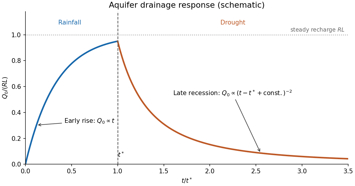
The curve illustrates these regimes and a possible . Its numerical shape and the relative duration of the regimes are schematic; the early rainfall and late drought formulas apply in their respective asymptotic ranges.
For a constant-mass density incompressible flow with no imposed body force, the two-dimensional Navier-Stokes equation isA conservative body force, if retained, may be incorporated into a modified pressure. Using scales and givesHere is the molecular kinematic viscosity. At high Reynolds number, inertia and the pressure gradient dominate on the outer length scale, while molecular viscous diffusion is small there. Thin boundary layers, narrow shear flows and fine turbulent scales can still have sufficiently large velocity gradients for viscous effects to matter. High Reynolds number permits instability and turbulence, but does not alone prove that every flow is turbulent. Molecular viscous dissipation remains essential at the small end of the turbulent cascade.
Write and , with . Assume a statistically stationary mean and sufficient regularity for Reynolds averaging to commute with spatial derivatives. Thenprovided the endpoint difference grows sublinearly. Averaging the continuity equation givesIn Einstein notation, the nonlinear term expands asThus the Reynolds-averaged Navier-Stokes equation isThe extra term survives because the average of a product of zero-mean fluctuations need not vanish; it represents turbulent transport of mean linear momentum.
The product rule and fluctuation incompressibility give the pointwise identityAveraging therefore givesThe fluctuation term is consequently the divergence of a Reynolds stress. The eddy viscosity model represents this momentum transport through a coefficient multiplying the mean strain-rate tensor:for its shear or deviatoric part. For example, in a thin parallel shear flow. The dynamic viscosity is an effective flow-dependent transport coefficient, rather than a molecular material property. Large eddies carry linear momentum between regions of different mean velocity.
There is a necessary qualification to the printed tensor equation (4). Taking its trace literally gives , which would exclude nonzero turbulence. A consistent deviatoric eddy-viscosity closure in fluctuating dimensions isThe isotropic term is absorbed into the effective pressure . Here for a strictly two-dimensional fluctuation model. The subsequent equations use for this effective pressure, or equivalently use (4) as a shear-stress closure. This preserves the intended thin-layer model without asserting an impossible full covariance identity.
For turbulent motions of scale and velocity scale , the estimate gives . It is much greater than one on energetic large scales and in the inertial range well above the Kolmogorov length scale. At the molecular dissipation scales it is no longer large, and molecular transport also dominates very near a smooth solid wall.
Let be a representative mixing-layer thickness, , and let be a representative streamwise velocity. Use the scalesThe transverse velocity scale follows from the mean continuity equation. For turbulent transverse transport to balance streamwise inertia,With this ordering, the streamwise eddy-stress divergence isThus transverse diffusion of streamwise linear momentum is retained, while streamwise diffusion and the contribution are smaller by . Molecular kinematic viscosity is neglected where .
In the transverse momentum equation, inertia and the retained eddy stresses have scale , whereas an order-one transverse pressure variation would give . Hence the leading dimensionless transverse balance is . The resulting boundary layer equations for the planar turbulent mixing layer areHere . The effective pressure convention explained in part (a)(iii) is understood. Since the outer streams have uniform horizontal velocities, their inviscid momentum equations give ; choosing the far-field gauge pressure as zero gives throughout this approximation.
Assume and set . With independent of , balancing streamwise transport with transverse mixing gives a layer width proportional to . Write its constant slope asHere is a spreading constant associated with the chosen definition of thickness; it is unrelated to the capillary in Question 1. The origin selects zero virtual-origin offset.
Define , , and introduce the stream functionThis automatically satisfies incompressibility and yieldsFor the momentum equation, use and :Because , the common coefficient cancels, giving the turbulent mixing-layer similarity equationThe boundary layer approximation also requires , consistently with the assumed slow spreading.
The two external stream velocities imposeLet and seek over . The nonlinear term is then , so the leading ordinary differential equation isFor , this is the first-order linear differential equation . Its integrating factor is , giving . An integration using the error function givesThe two far-field boundary conditions require and . A second integration usesConsequentlyThe relation between and cancels the extra term when differentiating. It gives the familiar error function mean velocity profileto first order in . The additive constant does not affect this velocity profile at the retained order; its interpretation comes from the transverse velocity.
For the approximate similarity profile, , and thereforeFor the prescribed undisturbed horizontal streams, a suitable choice is , which gives zero transverse velocity at both far-field limits. Then inside the layer. The nonzero internal crossflow is consistent with the streamwise widening of the velocity transition.
Another possible convention is to make the line a streamline, imposing . This requires , equivalently , and gives . It therefore requires a uniform outer crossflow relative to the coordinates used for the centred error function profile. A single constant cannot impose both zero far-field crossflow and unless . The physical lateral boundary conditions, or the chosen material centreline, determine which convention is appropriate. Since , these transverse velocities are of order for fixed .
Original solutions to the paper released at the source request. The complete editable transcription is retained in the private examination archive.
Choose vertically upward. Let be the gas-occupied part of a pipe cross-section, of area . Define the phase mean mass density, mass-weighted velocity, second moment of velocity, and phase mean pressure byThe void fraction is a volume fraction, not a mass fraction. The gas momentum in a slice of length is ; its advected momentum flux is . The two end pressures give the net force . Include every other vertical force on the gas, including interfacial forces, in . Newton's second law for this fixed slice, followed by division by , therefore givesThis is a cross-section averaged phase momentum balance. In particular, mass weighting makes the momentum and its flux exact averages; one must not replace by without an additional closure. With liquid mean velocity , constant liquid mass density , and liquid second moment , the same calculation givesWith the common pressure , the specified pressure contributions to cancel the phase-fraction derivatives from the product rule. The remaining pressure forces per unit mixture volume are and .
Assume that the bubbles at a given height have the stated radius . Their number per unit mixture volume is . The drag force on a rising bubble opposes its relative velocity, so multiplication of the single-bubble law by gives the signed magnitudeGravity acts downward; the drag force on the liquid is the opposite of that on the gas. With no wall force,A bubble retains its mass in the absence of transfer between phases. Consequently andFor clarity suppress bars on in the steady calculation. On a macroscopic variation length , gas inertia per unit volume scales like , whereas the quadratic drag force scales like . Their ratio is . Thus , together with the scale separation inherent in this averaging model, justifies the leading-order neglect of gas inertia. Small reference density alone does not justify it in an arbitrarily short or strongly compressed region. Neglect gas weight at the same order, with the liquid fraction not vanishing. For a stationary liquid, summing the two momentum equations givesThe leading gas balance is . Substitution of the bubble-radius law yieldsThe gas continuity equation, with constant pipe area and no mass exchange, is . Hence the steady gas mass flux is constant. For the pressure equation selects , andEvaluate the latter constant at a reference point , and divide. The terminal-drift density law for compressible bubbles isThe exponent comes from combining mass conservation with the density dependence of bubble radius; no gas equation of state was needed.
Existing answer advertised. Oxford’s Topics in Fluid Mechanics course archive lists “fhs 2010 q2 answer”, linked to the exact Question 2 answer resource. This question is skipped under the existing-answer policy. The advertisement was readable; the resource itself could not be fetched.
Write , and assume these scales are nonzero. The two reference liquidus relations imply . For the similarity variable and front ,Thus a temperature profile has and . Each heat equation becomes . The solute diffusion equation becomes , withThis Lewis number compares thermal and solutal diffusivities. Inside the mushy layer, gives . The wall and far-field conditions become and as .
At the moving phase boundary, equality of temperatures gives . Equality of concentrations gives . Therefore the dimensionless parameters with the convention used here areNeither concentration nor temperature offsets should be dropped when enforcing continuity. In particular can be negative. If , then : this is the inverse Stefan number, although the paper calls its Stefan number.
To check every factor of two in the flux conditions, divide the thermal Stefan condition by , and the solute balance by . This givesFinally and imply . This is marginal equilibrium at a mush-liquid boundary. Together these calculations produce all the rescaled differential equations and all three interface balances.
Integrating once gives . A second integration expresses the solution using the error function when the value at zero is prescribed, and the complementary error function when decay at infinity is prescribed. Write and take , . The wall condition and the interface value giveFor the exterior liquid, continuity at the interface fixes and . Thus the two decaying similarity solutions areThe factor is required because solute and heat diffuse on different length scales. Both denominators are positive for a finite positive . These formulas use the differential equations, wall/far-field data and continuity; the remaining three flux conditions determine their unknown constants.
Introduce three positive functions of the unknown front parameter:Differentiating the error function profiles gives , and at the interface. The three flux conditions are therefore exactlyThese undivided equations are the safest description of the constant-fraction mushy-layer similarity solution, including degenerate parameter choices. In the nondegenerate case the third equation first givesThe second then gives the solid fractionUse the third equation to replace the term in the first, and eliminate . The front parameter is a positive root of the single transcendental equationThen substitute back for and . Since the physical parameters have not been assigned numbers, an implicit scalar equation is the appropriate determination of .
The divided formulas require and . If either vanishes, return to the boxed three-equation system. For example gives , so the last equation demands ; otherwise this proposed similarity solution cannot exist. A physical branch must also have and . The algebra alone does not establish existence or uniqueness of such a branch for arbitrary parameters.
Original solutions to the paper released at the source request. The complete editable transcription is retained in the private examination archive.
Hydrostatic pressure varies with height as when the far flat bath is the zero-height reference. Surface tension balances that pressure jump by curvature; with the curvature sign chosen in the equation this becomes . Here is liquid mass density, gravitational acceleration, surface tension and the signed planar curvature. The capillary length balances these effects. Scale both physical and by to obtainFor the wall-rising meniscus decreases as rises. At the distant bath, , and , because the free surface becomes horizontal when expressed as . In the first integral this gives .
At zero wall contact angle the interface is tangent to the vertical wall. In the representation this means and , so . The rising contact point is . Put . Then . Integration from the contact point givesThe sign of is negative on the approach from below, while is positive, as required by the geometry. This local quadratic shape is the zero-contact-angle wall meniscus matching law.
Put , with physical transverse thickness . Matching the preceding quadratic meniscus gives when the inner amplitude is normalized as . After multiplying the transformed film equation by , its two capillary/gravity coefficients are and . Setting the curvature coefficient to one therefore givesThus the inner equation is exactly the stated . The leading matching conditions are as and a bounded film, with vanishing derivatives, as . They connect the static bath-side meniscus to a uniform entrained film.
For positive wall speed varying on the outer time scale, neglect the order- terms at leading order and setThe parabolic matching coefficient is unchanged because . Both remaining differential terms scale as , reducing the equation to . The supplied universal solution therefore yields the quasisteady drag-out matching lawAbove the turn-around region, and its outer derivatives are order one, while and . Hence the leading outer equation and inflow condition areThe boundary value comes from matching, not from setting the film to zero at the wall contact point.
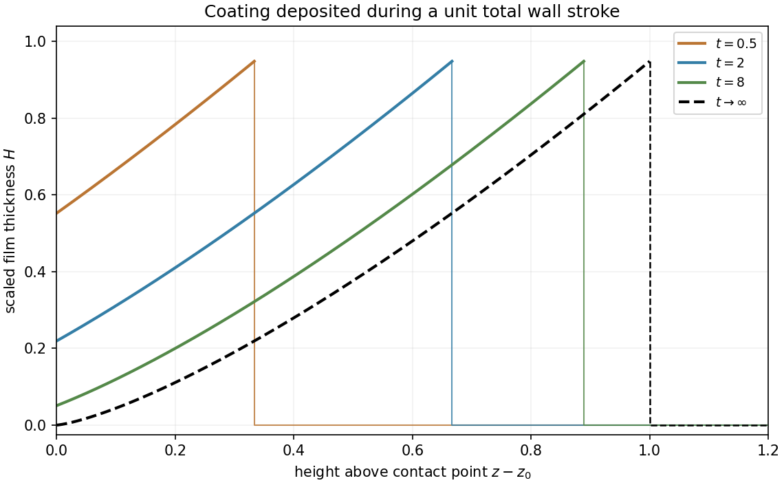
Along a characteristic, and . Integration gives , so . A characteristic entering through at time has and carries . Thus the boundary-fed and initially dry portions giveValues at are never sampled in the finite-time physical region and need not be prescribed. The moving coating front is . Explicitly,The incompatible initial corner creates a jump at the leading coating front; a trace convention at the jump does not affect the transported volume. The wall's total stroke is , so within this leading transport model the final profile isEarlier-deposited fluid is thicker and sits farther up the finite coated interval. Its total scaled volume is , agreeing with . This is a finite-stroke coating profile for the leading matched model.


Let equal one in phase one and zero in phase two; its interface value is immaterial for area integrals. In the absence of phase change or interfacial mass transfer, the distributional phase mass conservation is . For a cross-section of area , defineHere the symbol in the integral denotes the axial velocity component, not a derivative. Integrating through an arbitrary axial slice and using zero normal flux at the rigid pipe wall givesThe velocity is mass weighted, so the averaged mass flux factors exactly; an unweighted phase mean would not in general have this property. This is the cross-section averaged phase mass balance.
For phase two use , volume fraction , andThen . Mean quantities in a phase that is absent are unnecessary; the products giving conserved masses and fluxes remain the meaningful variables.
A spherical bubble displaces liquid volume . Neglect its own weight compared with the liquid buoyancy, as required by the stated gas/liquid approximation. Equating with the quadratic drag givesRetaining a nonnegligible gas density would add the factor . Let , so the upward slip is .
With constant phase densities, adding the two volume balances gives . The closed lower end fixes the total volume flux to zero. Solving it together with the slip relation yieldsIndividual bubbles move upward for , while small phase-fraction disturbances move at the characteristic speed . The latter is negative when : wave speed and bubble speed are different quantities.
A cleared region starts at the closed bottom, with and . Its Rankine-Hugoniot condition speed is . The intended clearing solution is thereforeIt is an entropy shock for the concave conservation law flux, since . Its speed also equals the bubble speed on its uncleared side, so it follows the last layer of bubbles. Under this continuation the last bubble reaches the outlet whenafter which throughout the pipe.
There is a boundary qualification for this dense initial mixture. The characteristics in the uncleared state point into the pipe from the top. To continue the displayed solution all the way to the stated clearance time, its incoming top trace must remain until clearing. Initial characteristics alone cover the shock only until , when its backward right-state characteristic first meets the top boundary. Atmospheric pressure by itself is not a boundary condition for this scalar phase-fraction equation. Thus the displayed formula and printed clearance time give the intended maintained-trace branch; a different top phase-fraction closure could change the later evolution. This is the incoming boundary condition in dense bubble clearing, and is separate from the local derivation of the conservation law.
Existing answer advertised. Oxford’s Topics in Fluid Mechanics archive lists “fhs 2009 q3 answer”, linked to the exact Question 3 answer resource. All three source subparts of this question are skipped under the existing-answer policy. The advertisement was readable; the resource fetch failed, so its contents were not inspected.
Original solutions to the paper released at the source request. The complete editable transcription is retained in the private examination archive.
The four dimensional equations express mass conservation, momentum balance with pressure, gravity and viscous stress, heat advection and conduction, and a linear thermal-expansion equation of state. For heating from below, suitable plate conditions are and at , and , at . No slip and thermal insulation on the sidewall provide one suitable lateral completion; prescribed lateral temperatures would be another specified thermal setup.
Let be thermal diffusivity and kinematic viscosity. Use , , and as length, time, velocity and temperature scales. Subtract the static reference pressure with and scale its remainder by . ThenDensity becomes . Substitution and division by the corresponding diffusion/viscous scales giveIn the Boussinesq small-density-contrast limit retain buoyancy while neglecting the other factors. At infinite Prandtl number, after any fast initial adjustment, the equations areThe velocity is instantaneously constrained by a viscous elliptic balance; the temperature still evolves.
Take the divergence of the vector Poisson equation. Derivatives commute, and divergence of a curl is zero, so . Its boundary value is zero, hence the maximum principle gives throughout . The vector identity now gives , orThe layer domain is simply connected because its horizontal section is simply connected. For a curl-free field on such a domain, define as its line integral from a fixed base point to . Contractibility of loops and Stokes theorem make the integral path independent, and differentiation gives its gradient equal to the field. Thus .
Incompressibility then gives , while the prescribed normal curl gives . Green's identity yieldsHence is constant on the connected domain and . The extra condition belongs to the stated potential boundary problem; the reconstruction argument above uses the divergence and normal-curl conditions. On a multiply connected domain a curl-free field need not be a globally single-valued gradient.
Finally . Taking the curl of the infinite-Prandtl momentum balance and using givesThe derivation is an instance of velocity reconstruction from a mixed-boundary vector Poisson problem.
The official course archive advertises an answer for this question. Its four parts are omitted from the original solutions under the existing-answer policy.
Define to be one in phase 1 and zero in phase 2, including its dependence on both transverse coordinates even though the averaged fields depend only on . With no interphase mass transfer, its distributional phase-mass equation is . At a pipe cross section of area , setThus is an intrinsic phase density and is the density-weighted mean axial velocity. This weighting is necessary when density varies within the phase; it becomes the ordinary intrinsic mean for an incompressible phase of constant density.
Integrate over the cross section. The transverse divergence contributes no boundary mass flux at the impermeable pipe wall, and the material interface has no mass leakage. The section area is constant, soFor phase 2 use and fraction , with the analogous intrinsic density and density-weighted velocity:The intrinsic quantities are defined where their phase fraction is nonzero. These are the intrinsic phase averages in a two-fluid pipe model.
Freeze a uniform state with , , and seek a finite characteristic speed . Denote its perturbation amplitudes by . The two phase-mass equations and two momentum equations giveEliminating the amplitudes givesWith , factor the quadratic over the complex numbers to obtainFor nonzero relative velocity the speeds are a nonreal conjugate pair. A Fourier perturbation on the growing branch has magnitude . Arbitrarily short waves therefore grow arbitrarily quickly, preventing a continuous dependence estimate in the usual finite-order Sobolev norms. This generic slip state is ill-posed as an initial value problem.
The pressure has no independent time-evolution equation; it enforces the incompressible volume constraint, so the request concerns the finite characteristic speeds rather than a freely propagating pressure mode. At the two speeds coincide and this particular nonreal-speed argument disappears; further degeneracy analysis is needed there, rather than calling coincident real speeds complex. The issue is complex characteristic speeds of a pressure-coupled two-fluid model.
For constant phase density, let be the intrinsic mean axial speed and defineThe profile coefficient measures the momentum flux relative to a uniform velocity profile with the same mean. Cauchy-Schwarz gives where the mean is nonzero, with equality for a uniform phase profile. At zero mean it is safer to retain the second moment itself rather than divide by .
In the stated common-pressure, no-extra-force closure, the averaged conservative momentum equation isFor constant , expand its derivatives and use . The terms combine asThereforeThis is the phase momentum profile coefficient correction. It accounts for the second moment of velocity, not merely a rescaling of the convective speed. A variable coefficient would also produce .
Articles were limited to the first 100 out of 101 total.
Articles by others on the same topic
There are currently no matching articles.