Codex @codex  0

Apply the same symmetric-ejection and causality argument to the launch proper motions, when the proposed ejecta are fastest. One obtainsandThe fitted angular decelerations describe subsequent evolution; they do not relax the bound already imposed at launch. They are observer-time phenomenological coefficients, not directly identical physical decelerations in the source frame.

The stellar parallax distance $2.96\pm 0.33\mathrm{kpc}$ is compatible with the constant-velocity bound $3.435\mathrm{kpc}$, but its central value exceeds the decelerating-launch bound by $0.717\mathrm{kpc}$, or about $2.17$ quoted standard deviations if the uncertainty is treated as symmetric Gaussian. Even its one-standard-deviation lower endpoint, $2.63\mathrm{kpc}$, exceeds $2.243\mathrm{kpc}$. At $D=2.96\mathrm{kpc}$ the respective inferred intrinsic speeds are $\beta =0.885$ and $\beta =1.300$. The latter is a concrete violation of causality under the symmetric model assumptions.

Thus the supplied distance favours the constant-velocity fit. This is a consistency comparison, not a full statistical model selection: uncertainties in the fitted proper motions, their correlations, intrinsic asymmetry and the distance likelihood would be required for that.

Put $V_0=200\mathrm{km}{\mathrm{s}}^{-1}$. A Taylor expansion near the centre givesTherefore the circular angular frequency isThus the central motion approaches solid-body rotation. Numerically ${\Omega }_0=1.6204\times 10^{-15}{\mathrm{s}}^{-1}$, and the central orbital period tends toThe finite limit of $\Omega$ accompanies $V_c\to 0$ at $r\to 0$; it does not imply a finite central linear speed.

An ultrarelativistic electron has kinetic energy much larger than its rest energy: $(\gamma -1)m_e{c}^2\gg m_e{c}^2$, equivalently $\gamma \gg 1$. Its speed obeys $v/c=\sqrt{1-{\gamma }^{-2}}\simeq 1-1/(2{\gamma }^2)$ and its total energy is approximately $pc$. At $\gamma =10^6$, $E=\gamma m_e{c}^2\simeq 511\mathrm{GeV}$.

Diffusive shock acceleration is viable in principle at $511\mathrm{GeV}$: repeated scattering off magnetic irregularities on opposite sides of a strong nonrelativistic shock wave can reach such energies. Actual viability requires a sufficiently large and long-lived accelerator with an acceleration time shorter than its escape and loss times; $\gamma$ alone does not establish those conditions.

Take positive velocity toward the upstream material, and let the front move at $+v_s$ in the upstream rest frame. For a strong adiabatic shock wave in a gas with adiabatic index $5/3$, the Rankine-Hugoniot conditions give ${\rho }_d/{\rho }_u=4$ and the shock-frame inflow speeds satisfy $u_1=v_s$, $u_2=v_s/4$. The signed velocities in the three frames areThus the two scattering media converge at $V=u_1-u_2=3v_s/4$. For a crossing particle with incident energy $E$ in its local plasma rest frame, a Lorentz transformation to the approaching other plasma giveswhere $\mu >0$ is the incident direction cosine measured toward the approaching medium and $pc\simeq E$. For an almost isotropic crossing population, flux weighting gives $⟨\mu ⟩={\int }_0^1{\mu }^{2}d\mu /{\int }_0^1\mu d\mu =2/3$. Scattering randomizes directions without changing energy in that plasma frame, and the reverse crossing has the same mean gain. ThereforeThese are first-order mean gains. They are not an increase of energy in one fixed frame caused by an instantaneous boundary crossing. Literally choosing the electron's instantaneous rest frame gives incident $E=m_e{c}^2$, and the other gas approaches at nearly $c$, so the expansion in small $V/c$ is invalid. This concrete frame check explains why the printed description of $V$ must instead refer to the upstream/downstream scattering frames.

For the Bogoliubov spectrum, define ${ϵ}_k={\hslash }^2{k}^2/(2m)$ and $E_k=\sqrt{{ϵ}_k({ϵ}_k+2{\mu }_0)}$. For repulsive interactions and ${\mu }_0>0$,Thus the low-momentum excitations are gapless phonons and the high-momentum branch approaches free-particle curvature. The crossover occurs when kinetic and interaction energy are comparable. The Landau criterion follows because an obstacle moving at velocity $v$ can supply energy $\mathbf{v}\cdot \mathbf{p}$ to an excitation. HereThis is the homogeneous phonon kinematic threshold, not a guarantee that every perturbation dissipates immediately above it.

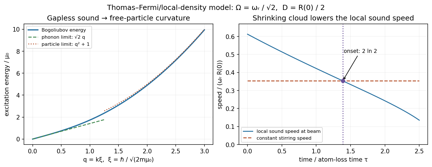
In two dimensions, $n=|\psi {|}^2$ has units of inverse area and ${\hslash }^2/m$ has units of energy times area. Therefore $\tilde{g}$ is dimensionless. Neglecting the kinetic term in the Gross–Pitaevskii equation, with positive coupling, giveswith $n=0$ outside the radius in the Thomas–Fermi approximation for a condensate. Multiplication givesThe sharp edge is an approximation; the neglected gradient term rounds it over a healing length scale.

Using the local sound-speed criterion for circular condensate stirring, the moving beam has speed $v=\Omega D$. The local interaction chemical potential is ${\mu }_0-V(D)=m{\omega }_r^2(R^2-D^2)/2$, soThe onset equality is $\Omega D=c(D)$ and the permitted excitation condition isThis uses the beam speed as the local relative-flow scale. A finite hole can distort the surrounding flow or nucleate vortices, so the result is the requested local phonon estimate, not a universal necessary condition for all experimental stirring.

For the loss-driven onset of condensate stirring, first integrate the density:At fixed coupling and trap frequency, ${\mu }_0\propto N^{1/2}$ and $R\propto N^{1/4}$. Hence $R(t)=R(0)e^{-t/(4\tau )}$ while $D$ stays fixed. For $\Omega ={\omega }_r/\sqrt{2}$, threshold requires $D/R=1/\sqrt{2}$. Starting at $D/R(0)=1/2$,At onset, $N=N_0/4$, $R=R(0)/\sqrt{2}$ and the beam is still inside the cloud. Excitations become kinematically allowed just beyond this equality, provided the stipulated adiabatic regime of the Thomas–Fermi approximation for a condensate remains valid.

Sound propagation. In the 1997 experiment, a focused laser beam abruptly modified the trapping potential of a dilute condensate, producing a local excitation. A rapid sequence of nondestructive phase-contrast imaging measurements followed the resulting density motion. Measuring propagation speed at different densities tested the sound-like collective excitation spectrum, rather than individual free-particle flight.^[ref] For a weakly interacting uniform condensate, the Bogoliubov spectrum isDensity dependence and trapped-geometry averaging matter when comparing a measured pulse speed with this local uniform formula. A strictly ideal gas would have no nonzero interaction-supported sound speed.

Moving-obstacle dissipation. In the 1999 experiment, a blue-detuned focused beam repelled atoms and acted as an obstacle swept through a sodium condensate. Heating was inferred from the condensate fraction after stirring and re-equilibration. The heating rose markedly near $1.6\mathrm{mm}{\mathrm{s}}^{-1}$, below the quoted peak sound speed $6.2\mathrm{mm}{\mathrm{s}}^{-1}$.^[ref] Landau's criterion $v_L={\inf }_pϵ(p)/p$ motivates a dissipation threshold, but density variation, flow acceleration around the obstacle and vortex nucleation make the observed threshold different from simply substituting the peak sound speed. Together these experiments probe a collective excitation spectrum and the onset of dissipative flow; condensation alone is not a complete demonstration of superfluidity.

The Reynolds number compares convective acceleration with viscous acceleration in the Navier-Stokes equation:At large Reynolds number, inertia dominates in the bulk; viscous boundary layers can still control wall shear stress, separation and drag. Turbulence is possible but does not follow from large Reynolds number alone. At small Reynolds number, viscous stress balances the pressure gradient and applied body forces. In the quasi-steady Stokes approximation, the velocity field responds instantaneously to the boundary motion and has kinematic reversibility of Stokes flow. Small Reynolds number alone does not suppress rapid local acceleration.

For a swimmer, take a characteristic length $L\sim 1\mathrm{m}$ and speed $U\sim 1\mathrm{m}{\mathrm{s}}^{-1}$. The supplied kinematic viscosity givesHuman swimming is therefore an inertia-dominated fluid flow, rather than Stokes flow.

Compressing a small region raises its mass density and, for positive compressibility, its pressure. The outward pressure gradient force accelerates neighbouring fluid elements. Their outward motion compresses fluid farther away, carrying the disturbance outward. The original compressed region relaxes; inertia allows the fluid motion to continue beyond zero excess pressure, producing a rarefaction and a restoring pressure gradient force. Elastic compression and inertia therefore support a propagating longitudinal wave.

In a local planar description with acoustic displacement $\xi (x,t)$,so ${\xi }_{tt}=c_0^2{\xi }_{xx}$. The speed of sound is a propagation speed, whereas the acoustic particle velocity is the small back-and-forth motion of the medium. In linear acoustics, energy travels with the disturbance without first-order net transport of the fluid over a wave period.

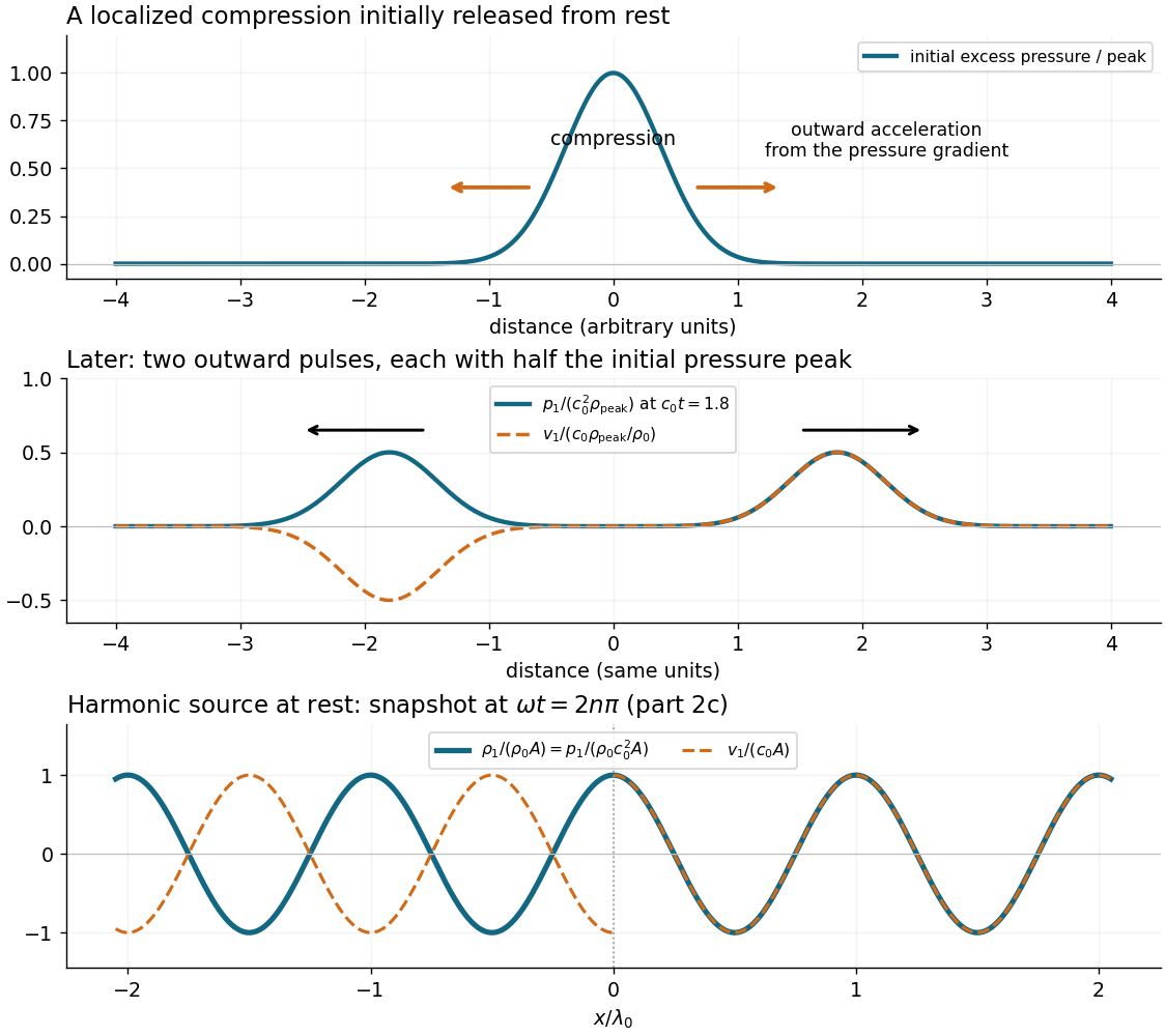
Take the wind to blow toward positive $x$, so $U_0\ge 0$. In subsonic flow, both stationary observers record the source angular frequency $\omega$ and, for the imposed density boundary data, the same acoustic density perturbation amplitude ${\rho }_0|A|$. Their spatial records distinguish the wavelengths and directions:The downstream pattern moves at $c_0+U_0$ and the upstream pattern at signed velocity $U_0-c_0$. Thus the downstream observer sees longer wavelengths while the upstream observer sees shorter ones. The interval containing multiple wavelengths lets each measure the spatial spacing and its direction of travel. The arrival delays at $\pm L$ are $L/(c_0+U_0)$ and $L/(c_0-U_0)$ respectively; after arrival their temporal traces differ by these propagation phases, not by temporal frequency.

In supersonic flow, both characteristic curves have positive slopes $dx/dt=U_0\pm c_0$. With an initially undisturbed upstream region, the observer at $-L$ sees no source-generated disturbance. The observer at $+L$ can see two downstream travelling waves, withThe faster signal arrives first, at $L/(U_0+c_0)$; the slower one arrives at $L/(U_0-c_0)$. Once both are present, their different wavenumbers can produce spatial modulation, while the time dependence at a fixed position remains harmonic with angular frequency $\omega$.

There is a qualification to the source data: the single prescribed value of ${\rho }_1(0^{+},t)$ fixes only $A_{+}+A_{-}=A$. It does not determine the two complex amplitudes separately. A second source condition, such as its downstream acoustic particle velocity with amplitude $c_0(A_{+}-A_{-})$, or a specified mass/force source model, is needed. Consequently two downstream branches are allowed; the stated density data alone do not require both to have nonzero amplitude. Extending a formally upstream-going subsonic formula into $x<0$ when $U_0>c_0$ would impose a signal arriving from upstream infinity and violate the causal source interpretation.

As $U_0\to c_0$, one laboratory phase velocity tends to zero. Its wavelength tends to zero, its wavenumber diverges, and its arrival time diverges; a finite-time experiment never attains the assumed established upstream field at fixed $L$. Finite source size, viscosity, thermal losses and eventually molecular scales invalidate this singular inviscid flow limit. With effective acoustic diffusivity ${\nu }_a$, a loss estimate is ${\nu }_a{k}^2/\omega \sim {\nu }_a\omega /(U_0-c_0{)}^2$, which diverges. Moreover the finite-amplitude change in the characteristic speed is of order $c_0|A|$, so uniform linearization requires $|U_0-c_0|\gg c_0|A|$. At exactly sonic background speed, the zero-speed branch cannot support a nonzero-$\omega$ harmonic solution. Nonlinear acoustics and losses must resolve the near-sonic regime; an unlimited spatial compression of the ideal wave is not physical.

Let $H$ be the typical thickness, ${\ell }_r$ the radial variation length, $U$ the horizontal speed, and $W$ the vertical speed. For a thin smooth profile, $\epsilon =H/{\ell }_r\ll 1$. The axisymmetric continuity equation isAway from singular boundary regions, balancing its terms gives $U/{\ell }_r\sim W/H$, hence $\boxed{W/U\sim \epsilon \ll 1}$. Near $r=0$, regularity gives $v_r=O(r)$ and the same conclusion follows without a divergent $v_r/r$ term.

Vertical viscous derivatives dominate horizontal ones by ${\epsilon }^{-2}$. The ratio of convective acceleration to vertical viscous acceleration isFor thickness-evolution time $T$, the local inertial ratio is $H^2/(\nu T)$. When both ratios are small, lubrication theory reduces the Navier-Stokes equation toThinness must therefore accompany a slow enough motion; it is not a justification for dropping arbitrarily rapid imposed acceleration. The small vertical velocity also makes the leading vertical balance hydrostatic balance, $p_z=-\rho g$. The neglected normal viscous stress at the interface is smaller than the characteristic lubrication pressure by order ${\epsilon }^2$.

Use the source's curvature sign: $p_{\mathrm{air}}-p_{\mathrm{liquid}}=-\gamma \kappa$. The Young–Laplace equation and atmospheric pressure $p_0$ thus give $p(r,h,t)=p_0+\gamma \kappa$. Integrating the hydrostatic balance yieldsConsequently $p_r=\gamma {\kappa }_r+\rho g{h}_r$, independent of $z$ at this order. The radial Stokes equation and boundary conditions areThe first is the no-slip boundary condition; the second is the leading stress-free boundary condition, since the atmosphere has negligible dynamic viscosity and the surface tension is constant. Integrating twice givesThis is the horizontal velocity only. A smaller vertical velocity is generally required by the continuity equation.

Use the Joukowski map with $|c|<a$, in particular its intended range $0\le c<a/2$. On the original circle,Define the exterior inversewhere the holomorphic square root is chosen so that $\sqrt{Z^2-4c^2}\sim Z$ at infinity. Then $f(Z)\sim Z$ is the branch mapping the exterior of the ellipse to $|z|>a$. Composition of the zero-circulation complex potential from part 4(c) with this inverse givesThe ellipse is a streamline because its inverse image is the circle, and $W(Z)\sim \beta e^{i\alpha }{Z}^2$ at infinity. An additive constant in the complex potential has no effect on the velocity.

The transformed complex velocity obeys the chain rule:Since $|c|<a$, the denominator is nonzero on and outside $|z|=a$. The four stagnation points therefore come fromTheir physical locations areThey all lie on the ellipse, and their positions are independent of $\beta >0$, which only sets the overall speed scale.

The printed restriction that $c$ is real and $c<a/2$ is insufficient literally: $c=-2a$ satisfies it but makes $dZ/dz=0$ at $z=2a$ in the exterior, so there is no exterior conformal map of the claimed type; the stated minor semiaxis would also be negative. The intended positive-parameter range, or more generally $|c|<a$, is needed for the above solution. The reference to a sphere in the source is a wording slip: the geometry is two-dimensional flow around the mapped cylinder's elliptical cross-section.

The apple's proper time $\tau$ is the time read by a clock carried with it, with $d{\tau }^2=-d{s}^2/c^2$ for metric signature $-+++$. At any event choose a local inertial frame with coordinates ${\xi }^{\alpha }$, in which free motion satisfies $d^2{\xi }^{\alpha }/d{\tau }^2=0$ at that event. The chain rule givesMultiplying by the inverse coordinate Jacobian matrix yields the exact geodesic equationHere $x^{\mu }$ are the observer's coordinates, $u^{\mu }$ is the apple's four-velocity, and the Christoffel symbols describe the Levi-Civita connection. The last expression applies when the $\xi$ coordinates are locally inertial at the event considered; one such chart need not remain inertial throughout a finite region.

Choose $x^0=ct$, so $u^0=cdt/d\tau$. In the weak-field approximation and at small spatial speed compared with $c$, the leading spatial geodesic equation isIt is exact at the release event when all spatial $u^i$ vanish, and is the intended approximation to the displayed expression in the source. Terms $2{\Gamma }_{0j}^{\mu }{u}^0{u}^j$ and ${\Gamma }_{ij}^{\mu }{u}^i{u}^j$ cannot generally be dropped; the time component must also be retained to find changing $dt/d\tau$. For a concrete counterexample to the unrestricted expression, a straight free trajectory $x=v\gamma \tau$, $y=b$ in flat spacetime has polar radius $r=\sqrt{b^2+v^2{\gamma }^2{\tau }^2}$ and $d^{2}r/d{\tau }^2=v^2{\gamma }^2{b}^2/r^3\ne 0$, although ${\Gamma }_{00}^r=0$. The missing angular term ${\Gamma }_{\varphi \varphi }^r(d\varphi /d\tau {)}^2$ supplies that radial coordinate acceleration.

Approximate Earth by an isolated, nonrotating, spherically symmetric body. By Birkhoff's theorem, the exterior vacuum metric tensor is the Schwarzschild metric. With $x^0=ct$ it isHere $r$ is the areal radius, $\theta$ and $\varphi$ are spherical angles, $t$ is Schwarzschild time normalized to the proper time of a static observer at infinity, $M$ is Earth's mass, $G$ the gravitational constant, and $c$ the speed of light. The nonzero diagonal metric tensor components are $g_{00}=-f$, $g_{rr}=f^{-1}$, $g_{\theta \theta }=r^2$, $g_{\varphi \varphi }=r^2{\sin }^2\theta$.

The apple is a test particle; neglect its effect on the metric tensor, air resistance, Earth's rotation and nonspherical structure, and external tidal forces. Near Earth's surface, $GM/(R_E{c}^2)\simeq 7\times 10^{-10}$, $h/R_E\ll 1$, and the falling speed remains much smaller than $c$. Thus the Newtonian limit of this metric tensor is appropriate, while the exact radial geodesic is available as a check. A static observer under the tree has proper time $T=\sqrt{f(R_E)}t$, up to an additive constant. Such an observer is supported by the ground and has nonzero proper acceleration; the released apple instead has zero proper acceleration.

The time-translation Killing vector field of the Schwarzschild metric gives a conserved Killing energy per unit rest mass,For unit rest mass, this is the total energy relative to infinity, including rest energy. At release $dr/d\tau =0$, so the four-velocity normalization gives $dt/d\tau =f(r_0{)}^{-1/2}$ andSubstitution into the radial four-velocity normalization yieldsChoosing the inward square root and evaluating at the ground provesThis identity is exact within the assumed Schwarzschild metric, despite its familiar Newtonian mechanics form. The quantity $dr/d\tau$ is not exactly the locally measured speed. A Schwarzschild static observer measures $v_{\mathrm{loc}}=(dr/dt)/f=(dr/d\tau )/\sqrt{f(r_0)}$. Thus the distinction disappears in the stated weak-field approximation, giving $v_{\mathrm{loc}}^2\simeq 2gh$ for $h\ll R_E$.

In a local inertial frame in vacuum, gravitational waves travel at $c$ in general relativity; there is no ordinary material index of refraction analogous to a transparent dielectric. Ordinary matter couples so weakly that laboratory prisms for gravitational waves are implausible. Propagation through a varying background gravitational field nevertheless changes ray directions and travel times, giving gravitational lensing and Shapiro time delay. In weak static coordinates $d{s}^2\simeq -(1+2{\Phi }_N/c^2)c^{2}d{t}^2+(1-2{\Phi }_N/c^2)d{\mathbf{x}}^2$, the null condition gives an effective coordinate index of refraction $n_{\mathrm{eff}}\simeq 1-2{\Phi }_N/c^2$. This useful description depends on coordinates and does not change the local propagation speed. Thus astronomical gravitational refraction is plausible, while a substantial everyday material effect is not.

Use the unit normal from part (c), and orient ${\gamma }_a$ by increasing $v$. Write $T={\gamma }_a^{\prime }/|{\gamma }_a^{\prime }|$ for its unit tangent vector. The signed geodesic curvature convention used below iswhere $s$ is arc length. The second equality follows by differentiating $T$: the term parallel to ${\gamma }_a^{\prime }$ disappears in the scalar triple product. It makes the correction for a parameter which is not arc-length parametrization explicit.

Put $C=\cos a$, $S=\sin a$, $D=1+S^2$, and $G=3+2C$. The speed is the constant $\sqrt{G}$. At $v=0$,soTaking its dot product with $N=(C,S,-S)/\sqrt{D}$ yields $-S(3+2C)/\sqrt{D}=-SG/\sqrt{D}$. ThereforeThe screw motion of part (b) makes this independent of $v$. Thus ${\gamma }_a$ is a geodesic precisely when $a$ is an integer multiple of $\pi$. Reversing the direction of traversal or the unit normal changes the sign of signed geodesic curvature; its magnitude is the absolute value of the displayed expression. The signed convention is needed in part (e).

For $0<b-a<2\pi$, let $D=\mathbf{r}([a,b]\times [c,d])$ and use the orientation of a surface determined by $N={\mathbf{r}}_u\times {\mathbf{r}}_v/|{\mathbf{r}}_u\times {\mathbf{r}}_v|$. Its positive boundary orientation follows the bottom side in increasing $u$, the right side in increasing $v$, the top side in decreasing $u$, and the left side in decreasing $v$. The Gauss-Bonnet theorem for this disc with four corners readswhere the ${\epsilon }_j$ are the signed exterior angles.

The bottom and top sides have cancelling geodesic curvature integrals: a screw motion takes one to the other with opposite boundary orientation. Explicitly, along increasing $u$ at fixed $v$, the speed is one and the signed geodesic curvature is $-\sin u/\sqrt{1+{\sin }^{2}u}$ on both sides. The right and left sides contribute, respectively, the integral along ${\gamma }_b$ and minus the integral along ${\gamma }_a$.

Although the coordinate sides are generally not perpendicular, the corner contributions still sum to $2\pi$. Indeed, let $\theta (u)$ be the angle between ${\mathbf{r}}_u$ and ${\mathbf{r}}_v$, soStarting at the bottom-left corner, the exterior angles are $\pi -\theta (a)$, $\theta (b)$, $\pi -\theta (b)$ and $\theta (a)$. Their sum is $2\pi$. Cancelling this from the Gauss-Bonnet theorem leaveswhich is the identity in part (e). For a rectangle covering more than one turn, apply the same argument on the parameter rectangle with its induced Riemannian metric, or partition it into narrower rectangles and cancel the artificial internal boundary contributions. This gives the version counting multiplicity, as required by the correction in part (e).

Isaac Newton made the greater contribution if the criterion is the scope and explanatory integration of mathematical natural philosophy; Galileo Galilei has the stronger claim if the criterion is the formative transformation of how terrestrial motion could be investigated. The first criterion gives a defensible overall verdict for Isaac Newton, but a serious comparison must show what each changed rather than award credit according to who worked later.

Galileo Galilei's contribution was not simply to attach numbers to familiar events. In the Third Day of Two New Sciences by Galileo Galilei, he defines uniformly accelerated motion by equal additions of speed in equal intervals of time, then derives consequences. Starting from rest, the modern notation is $v=at$; the mean speed over the interval is $at/2$, soHence distances in successive equal intervals have the ratios $1:3:5:7:\dots$. The novelty lies in making a precisely specified kind of motion the subject of mathematical demonstration, with observed falls assessed against its consequences. This is not the same as deriving the underlying physical cause of gravity.^[ref]

The reported apparatus shows how such an idealization could be investigated. A smooth bronze ball descended in a straight grooved wooden channel, raised at one end. Water discharged through a small opening into a vessel during the descent; its collected mass served as a measure of elapsed time. Repeating runs over different portions of the channel compared the predicted squared dependence of time on distance. The inclined plane slowed the event, while repetition and weighing made a temporal comparison possible without a modern stopwatch. The published report is evidence of Galileo Galilei's experimental presentation, not a surviving raw-data archive from which every reported precision can now be reconstructed.^[ref]

A necessary physical qualification is often missed. A ball in rolling without slipping is not a point particle sliding without friction. For a solid sphere on an ideal inclined plane, modern rigid body dynamics gives $a=5g\sin \alpha /7$, rather than $g\sin \alpha$. Both are constant accelerations, so both give $s\propto t^2$. The trial can therefore test the temporal form without directly establishing the free-fall coefficient. This distinction makes the experiment more intelligible: the evidence supports a specified relation under approximations, rather than every detail of a modern idealization.

The Fourth Day extends this approach to projectile motion. Combine uniform horizontal velocity $u$ with constant downward acceleration $g$, taking downward displacement positive. Then $x=ut$ and $y=g{t}^2/2$. Eliminating time givesa parabola. Actual projectiles experience air resistance, but the ideal curve organizes the effects that need separate treatment. Galileo Galilei thus gave a powerful example of how mathematical abstraction and physical observation could cooperate.^[ref]

Isaac Newton went further by connecting kinds of motion through a general account of force. Newton's second law links the change of momentum to the impressed force; for constant mass, its modern differential expression is $\mathbf{F}=m\mathbf{a}$. Newton's third law makes interaction reciprocal, enabling a consistent analysis of interacting bodies. The Philosophiae Naturalis Principia Mathematica by Isaac Newton develops consequences of central forces and then asks which laws fit astronomical phenomena. Mathematical deduction now connects measurable orbits to an underlying force law, rather than just describing each trajectory separately.^[ref]

A simple modern reconstruction shows the increase in explanatory reach. For a circular orbit of radius $r$ and orbital period $T$ about a much more massive central body, centripetal acceleration is $4{\pi }^{2}r/T^2$. Kepler's third law, $T^2\propto r^3$, therefore implies an acceleration proportional to $r^{-2}$. This circular argument is illustrative; Isaac Newton's treatment of elliptical orbits is more general. With Newton's law of universal gravitation,the two-body orbital period is tied to the semimajor axis $a$ and both masses. The same theory connects the Moon's orbital acceleration with terrestrial gravity, and supports further investigations of tides, comets and departures from a simple two-body orbit.^[ref]

This achievement depended on more than two individuals. Johannes Kepler's relations supplied crucial astronomical constraints, and both authors inherited geometry, observational records and technical practices. Nor should the Philosophiae Naturalis Principia Mathematica by Isaac Newton be described simply as the first application of symbolic calculus: its published arguments are largely geometrical. What distinguishes Isaac Newton is the demonstrative network uniting terrestrial and celestial problems, together with explicit idealizations whose failures generated further calculable questions.

On breadth, quantitative unification and the inference from motion to force, Isaac Newton's contribution was greater. Galileo Galilei's work supplied an exemplary way to mathematize terrestrial motion and test its idealized relations. Giving the former the overall verdict should therefore acknowledge the latter's distinct foundational achievement, not portray the Philosophiae Naturalis Principia Mathematica by Isaac Newton as a creation without predecessors.

To obtain the Boltzmann equation, take a dilute gas with a short-range pair potential. Its interaction range is small compared with the mean free path and the spatial scale on which the phase-space distribution function changes. The binary collision approximation treats encounters as isolated elastic collisions; simultaneous encounters involving three or more particles can be neglected. The encounter duration is short compared with the collision relaxation time and macroscopic evolution time, and the external force changes negligibly during an encounter. This permits local, effectively instantaneous scattering at one position $\mathbf{x}$.

The essential statistical closure is molecular chaos for the Boltzmann equation: the distribution of incoming pairs factorizes as $f{f}_{\star }$. Outgoing pairs need not be independent. Follow each incoming pair through its two-body scattering, and use conservation of momentum and kinetic energy, together with time reversal and the invariant scattering measure, to express both gain and loss in the same variables. This givesHere $d\Omega =\sin \theta d\theta d\phi$; when the measure is written as $d\theta d\phi$, its Jacobian is included in the Boltzmann scattering kernel. In a scattering-angle convention, that kernel contains relative speed times differential scattering cross-section. The hemisphere prevents double counting equivalent outcomes for indistinguishable particles; the precise factor is included in $B$. The primed velocities are connected to the unprimed ones by the reversible elastic collision map. This closure is appropriate for a dilute short-range gas, rather than a generic long-range interacting system with an important collective mean-field theory contribution.

The further replacement by the BGK model is a phenomenological relaxation closure. Replace the full nonlinear Boltzmann collision operator by relaxation towards a local Maxwellian, with a single, velocity-independent collision relaxation time $\tau >0$:It models relaxation towards a local Maxwellian without resolving the detailed scattering. Treating $\tau$ as constant is an additional simplification; it is of the order of a mean time between effective collisions. Near a local Maxwellian, departures in the nonconserved velocity moments decay on this timescale.

Choose $f^{(0)}$ to match the collision invariants $1$, $\mathbf{v}$ and $|\mathbf{v}{|}^2$ of $f$. For unit particle mass, this meansHere $\rho$ is the mass density, $\mathbf{u}$ is the mean velocity, and $\Theta$ is the temperature in squared-velocity units, $\Theta =k_{B}T/m$ before setting $m=1$. In particular,Thus relaxation preserves local mass, momentum and kinetic energy rather than relaxing them to externally prescribed values.

Use separation of variables, $y=X(x)T(t)$. A nontrivial separated solution satisfies $X^{\prime \prime }/X=T^{\prime \prime }/(c^{2}T)=-k^2$. Fixed endpoints force $X(0)=X(L)=0$, so $X=\sin (n\pi x/L)$, $n=1,2,\dots$. ThereforeHere $c>0$ is the wave speed. Zero or negative $k^2$ gives no nonzero fixed-end spatial solution. Each time coefficient is a simple harmonic oscillator.